N-Dimensional Generalization of Linearized Gaussian Fitting
Papers by [Anthony-Granick] and [Wan-Wang-Wei-Li-Zhang] naturally focus on the two-dimensional case of Gaussian fitting presented in image analysis. In fact, neither paper regards axis cross-coupling terms in their representations, instead focusing on unrotated ellipsoids.
The goal of this segment is to demonstrate a solution with the cross-coupling term in two dimensions, and then generalize to arbitrary number of dimensions. The mathematics of this article is very basic, but the final result is both useful and interesting for practical applications.
Adding a Cross-Coupling Term
Both papers do not go past expressing a Gaussian as
(65)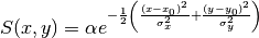
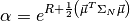
The complete equation, with a rotated error ellipse requires an additional
cross-coupling term  :
:
(66)
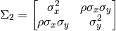
This particular formulation is derived by inverting a 2x2 covariance matrix
with cross-coupling term :
(67)
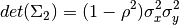
The determinant of this matrix is given by
(68)
The inverse covariance matrix is therefore
(69)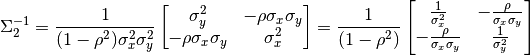
It should be clear how this matrix translates to (66). If not, see the generalization in Expanding to Arbitrary Dimensions, which expounds the details more exhaustively.
If we linearize (66) by taking the logarithm of both sides and aggregate the coefficients, we get
(70)
Here  is shorthand for
  , and the parameters have been
combined as follows:
, and the parameters have been
combined as follows:
(71)
This equation is in a form suitable for a direct least-squares estimation of
the parameter values, as long as we have at least six data samples
 available to ensure a fully determined problem. Based
on the papers that this algorithm is extending, we will want to add weights to
the solution as well. The exact nature of the weights is out of scope for this
article. Suffice it to say that we have individual weights
available to ensure a fully determined problem. Based
on the papers that this algorithm is extending, we will want to add weights to
the solution as well. The exact nature of the weights is out of scope for this
article. Suffice it to say that we have individual weights  for each
sample. Our goal is to find the projection that minimizes the error for the
following matrices:
for each
sample. Our goal is to find the projection that minimizes the error for the
following matrices:
(72)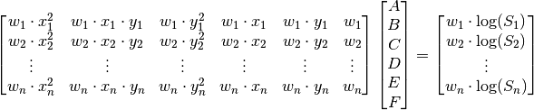
Any of the common linear algebra solvers should be able to solve this least squares problem directly.
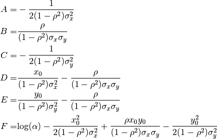
Rather than attempting to express the six parameters  ,
,  ,
,
 ,
,  , and
, and  directly in
terms of ,
directly in
terms of ,  ,
,  ,
,  ,
,  ,
,  , let
us search for a solution for , , and the elements of
, let
us search for a solution for , , and the elements of
 as given in (69) instead. Not only will
this be simpler, but the generalization to mutliple dimensions will be more
apparent.
as given in (69) instead. Not only will
this be simpler, but the generalization to mutliple dimensions will be more
apparent.
(73)
We can notice that the coefficients for and in the
equations for and have the form
(74)
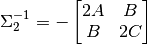
Inverting this matrix and working out the terms divided by the determinant gives us
(75)
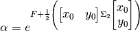
Finally, we can solve for the amplitude  by rewriting the
equation for as
by rewriting the
equation for as
(76)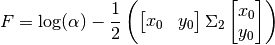
The amplitude is given by
(77)
We can extract , , and from
 , but as the next section shows, this is not practically
necessary.
, but as the next section shows, this is not practically
necessary.
Expanding to Arbitrary Dimensions
A multivariate Gaussian is characterized by its amplitude ,
covariance matrix  , and location
  :
:
(78)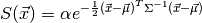
Since is the positive definite matrix, we only need to specify
the upper half of it. A least squares fit to an N-dimensional Gaussian will
therefore always have  parameters from the
covariance matrix,
parameters from the
covariance matrix,  from the location, and one from the amplitude, for
a total of
from the location, and one from the amplitude, for
a total of  parameters. This is consistent
with the six-parameter fit for a 2-dimensional Gaussian show in the previous
section.
parameters. This is consistent
with the six-parameter fit for a 2-dimensional Gaussian show in the previous
section.
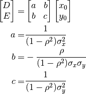
We can group our coefficients into two parameter vectors and a scalar:
 is the vector of coefficients of the covariance terms,
 is the vector of coefficients for the location terms, and
 determines the amplitude. For the two dimensional case shown in
(71), we have
determines the amplitude. For the two dimensional case shown in
(71), we have
(79)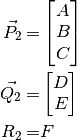
Since  is a multidimensional quantity, let us denote the
 th component with a left subscript:
  . The matrix
equation that generalizes (72) for N dimensions then becomes
. The matrix
equation that generalizes (72) for N dimensions then becomes
(80)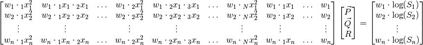
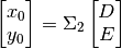
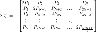
The solution is then a generalized form of each of (73),
(75) and (77). First we ravel
to make the inverse of :
(81)
We can then find the location from the portion:
(82)
And finally the amplitude:
(83)