_reei-supplement:

Supplementary Materials¶

Additional Considerations
Extended Applications
- Three-Parameter Gaussian
Errata

The purpose of this translation was originally to motivate the writing of the scikit to which it is attached. As such, the calculations shown for linear regressions in the paper can be greatly simplified using the power of existing linear algebra solvers. The particular implementations discussed in this section are targeted towards numpy and scipy in particular. However, the formulation shown here will most likely be helpful for a number of other modern linear least-squares packages. This is especially true since many software packages, including numpy and scipy, share LAPACK as a backend for performing the actual computations.

With a linear algebra package such as LAPACK, it is sufficient to compute the coefficient matrix $M$ and ordinate vector $p$ , without performing any further operations on them. A linear regression is generally solved as something equivalent to

$x = \left( M^T * M \right)^{-1} \left( M^T * p \right)$

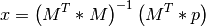
The formulae in the paper show how to compute the elements of $M^T * M$ and $M^T * p$ , which is usually done more efficiently by existing packages when given the raw $M$ and $p$ . These variable names were chosen to avoid conflict with the names $A$ , $B$ , $a$ , $b$ , etc, which are used heavily by the paper and software package documentation for different things.

The following sections show how to construct such simplified solutions to the equations in the paper. Solutions are described briefly, and presented concretely with Python code. The solutions here are for conceptual reference only. They are not a complete or exact reflection of how things are done in the scikit itself. The scikit makes an effort to optimize for speed over legibility, which does not suit the purpose of this exposition.

In the code snippets below, x and y are assumed to be one-dimensional numpy arrays. Both arrays have an equal number of elements, n. Numpy is implicitly imported under the conventional name np. The solution to each regression can be obtained by running one of the following two function calls:

params, *_ = scipy.linalg.lstsq(M, p)
params, *_ = numpy.linalg.lstsq(M, p)

Gaussian PDF ¶

Algorithm originally presented in 3. Example: Illustration of the Gaussian Probability Density Function and summarized here.

$M$ is a matrix with the cumulative sums $S$ and $T$ as the columns. In numpy terms:

d = 0.5 * np.diff(x)

S = np.cumsum((y[1:] + y[:-1]) * d)
S = np.insert(S, 0, 0)

xy = x * y
T = np.cumsum((xy[1:] + xy[:-1]) * d)
T = np.insert(T, 0, 0)

M = np.stack((S, T), axis=1)

$p$ is the vector of measured $y$ values decreased by its first element. In numpy terms:

p = y - y[0]

Gaussian CDF ¶

Algorithm originally presented in Appendix 2: Linear Regression of the Gaussian Cumulative Distribution Function and summarized here.

$M$ is a matrix with just the $x$ values and ones as the columns. In numpy terms:

M = np.stack((x, np.ones_like(x)), axis=1)

$p$ is a more complicated function of $y$ in this case:

p = scipy.special.erfinv(2 * y - 1)

Exponential ¶

Algorithm originally presented in 2. Regression of Functions of the Form y(x) = a + b \; \text{exp}(c \; x) and summarized here.

In the first regression to obtain the parameter $c$ , we have for $M$ :

d = 0.5 * np.diff(x)

S = np.cumsum((y[1:] + y[:-1]) * d)
S = np.insert(S, 0, 0)

M1 = np.stack((x - x[0], S), axis=1)

$p$ is the vector of measured $y$ values decreased by its first element. In numpy terms:

p1 = y - y[0]

Once we find a fixed value for $c_1$ (as the variable c1), we can fit the remaining parameters with $M$ constructed from $c_1$ and $x$ . In numpy terms:

M2 = np.stack((np.ones_like(x), np.exp(c1 * x)), axis=1)

$p$ is just the raw $y$ values for this regression. In numpy terms:

p2 = y

Weibull CDF ¶

Algorithm originally presented in 3. Regression of the Three-Parameter Weibull Cumulative Distribution Function and summarized here.

This is just a transposed and transformed version of the Exponential case. The input $x$ and $y$ are first swapped, and then the new $x$ values are transformed according to (34). In numpy terms:

x, y = np.log(-np.log(1.0 - y)), x

Sinusoid with Known Frequency ¶

Algorithm originally presented in 2. Case Where \omega is Known A-Priori, in equation (42). The algorithm is not summarized in detail since it deals with a trivial case that is not particularly useful in practice.

The matrix $M$ is a concatenation of the final coefficients in (41). Assuming that the angular frequency $\omega_e$ from the equations is given by the Python variable omega, we have:

t = omega * x
M = np.stack((np.ones_like(x), np.sin(t), np.cos(t)), axis=1)

$p$ is just the vector of raw $y$ values for this regression. In numpy terms:

p = y

Integral-Only Sinusoidal Regression Method ¶

Algorithm originally presented in 3. Linearization Through an Integral Equation, in equation (51). This equation consitutes the first step in the complete process summarized in Appendix 1: Summary of Sinusoidal Regression Algorithm and detailed in Appendix 2: Detailed Procedure for Sinusoidal Regression.

$M$ is a matrix constructed from the second-order cumulative sum $SS$ and powers of $x$ :

d = 0.5 * np.diff(x)

S = np.cumsum((y[1:] + y[:-1]) * d)
S = np.insert(S, 0, 0)

SS = np.cumsum((S[1:] + S[:-1]) * d)
SS = np.insert(SS, 0, 0)

M = np.stack((SS, x**2, x, np.ones_like(x)), axis=1)

$p$ is just the vector of raw $y$ values for this regression. In numpy terms:

p = y

Further Optimization of Sinusoidal Phase and Frequency ¶

The additional optimization step presented in 5. Further Optimizations Based on Estimates of a and \rho, in equation (57). This equation consitutes the second step in the complete process summarized in Appendix 1: Summary of Sinusoidal Regression Algorithm and detailed in Appendix 2: Detailed Procedure for Sinusoidal Regression.

$M$ for a purely linear regression is just ones and $x$ concatenated column-wise:

M = np.stack((x, np.ones_like(x)), axis=1)

$p$ is less trivial, since it the vector $\theta$ , shown in (56). This computation assumes that we already have estimates for $a_1$ , $b_1$ , $c_1$ and $\omega_1$ stored in the variables a1, b1, c1 and omega1 from the previous step in the algorithm:

rho1 = np.hypot(c1, b1)
phi1 = np.arctan2(c1, b1)

f = y - a1
dis = rho**2 - f**2
m = (dis >= 0)
Phi = np.arctan(np.divide(f, np.sqrt(dis, where=m), where=m), where=m)
np.copysign(np.pi / 2.0, f, where=~m, out=Phi)

kk = np.round((omega1 * self.x + phi1) / np.pi)
theta = (-1)**kk * Phi + np.pi * kk

p = theta

Due to limitations in numpy, kk must be a floating-point datatype for the expression (-1)**kk to work properly. Any negative values in kk would raise ValueError: Integers to negative integer powers are not allowed.

Final Optimization of Sinusoid Once Frequency is Found ¶

The final optimization step is presented in 6. Final Steps and Results, in equation (59). This equation consitutes the third step in the complete process summarized in Appendix 1: Summary of Sinusoidal Regression Algorithm and detailed in Appendix 2: Detailed Procedure for Sinusoidal Regression.

We assume that the optimized value $omega_2$ is stored in the variable omega2 to compute $M$ :

t = omega2 * x
M = np.stack((np.ones_like(x), np.sin(t), np.cos(t)), axis=-1)

$p$ is just the vector of $y$ values:

p = y

Computation and Plotting of Randomized Figures ¶

Some of the figures in the paper contain too many data points to place conveniently in a table. In such cases, the translation attempts to reproduce the results with randomly generated data following the paper’s instructions. The number of points used in such cases is sufficient to allow all the results to match within acceptable thresholds.

Reference implementation of the code used to generate the various radomized figures and tables is shown below, along with brief explanations. The figures are regenerated every time the documentation is built, so results will always vary slightly.

Cumulative Distributions and Medians ¶

In measuring the accuracy of the sinusoidal regression algorithm, a number of figures showing cumulative distributions of a ratio of anglar frequencies is used for demonstration: in Fig. 9, Fig. 10, reei-sin-h-plot, reei-sin-i-plot and reei-sin-k-plot. The code to simulate $N$ fits with $n_p$ (n in the code ) points per period goes something like this:

omega_e = 2.0 * np.pi
x = np.random.rand(N, n)  # One simulation per row
x.sort(axis=1)
y = np.sin(omega_e * x)

omega = [self.fit(*k) for k in zip(x, y)]

Here fit is a function that accepts the $x_k$ and $y_k$ vectors and returns an estimate for $\omega$ . The exact function will differ depending on whether we are discussing $\omega_1$ , $\omega_2$ or $\omega_3$ . For sufficiently large $N$ , there is a good likelihood that the values of $\omega$ will contain NaN due to pathological input data (where $\sqrt{-A_1}$ is imaginary), so we filter the list:

ratios = np.array([f / omega_e for f in omega if not np.isnan(f)])

The loss of one or two elements for very large $N$ will not affect the PDF and CDF much:

pdf, bins = np.histogram(ratios, bins=500, density=True)
pdf *= np.diff(bins)                # Convert density into mass
bins = 0.5 * (bins[1:] + bins[:-1]) # Use bin centers
cdf = np.cumsum(pdf)

The median value of the distribution is obtained through linear interpolation:

med = np.interp(0.5, cdf, bins)

Extended Applications ¶

Some additional common functions and modifications that can be added to the suite presented in the paper are presented here.

Three-Parameter Gaussian ¶

In the real world, data often comes out as an unnormalized Gaussian of three, rather than two parameters, with the third parameter being the amplitude or normalization. The normalization constant of the Gaussian PDF is chosen so that the total area under the curve is unity:

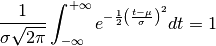
$\frac{1}{\sigma \sqrt{2 \pi}} \int_{-\infty}^{+\infty} e^{-\frac{1}{2} \left(\frac{t - \mu}{\sigma} \right)^2}dt = 1$

The amplitude of the PDF at the peak $x = \mu$ is therefore $\frac{1}{\sigma \sqrt{2 \pi}}$ . An unnormalized Gaussian can be conveniently parametrized either in terms of its total area $A$ , or peak amplitude $a$ , in addition to $\mu$ and $\sigma$ . We have the relationship:

$a = \frac{A}{\sigma \sqrt{2 \pi}}$

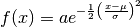
Either is a valid choice for the third parameter. The scikit uses the amplitude $a$ because it is easier to visualize, and makes the computation just a little easier. We therefore wish to use the methodology presented in the original paper to find the parameters $a$ , $\mu$ and $\sigma$ which optimize the fit to some set of data points $(x_1, y_1), (x_2, y_2), ..., (x_k, y_k), ..., (x_n, y_n)$ of our function:

$f(x) = a e^{-\frac{1}{2} \left(\frac{x - \mu}{\sigma} \right)^2}$

The formulation of the integral equation (3) is still applicable because the amplitude parameter is not resolvable from those equations. We are able to solve for the approximations $\mu_1$ and $\sigma_1$ as before (but with a different $f(x)$ , which absorbs the multiplicative constant).

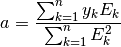
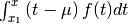
Optimizing $a$ will require an additional step. Fortunately, with $\mu$ and $\sigma$ fixed, the minimization of residuals in terms of $a$ is already a linear problem:

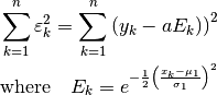
$\sum_{k=1}^n \varepsilon_k^2 = \sum_{k=1}^n \left(y_k - a E_k)\right)^2 \\ \text{where} \quad E_k = e^{-\frac{1}{2} \left(\frac{x_k - \mu_1}{\sigma_1} \right)^2}$

Setting the partial derivative of the sum of squared errors with respect to $a$ to zero:

$\sum_{k=1}^n \left( y_k - a E_k \right) E_k = 0$

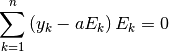
Since we are solving for only one unknown, a single equation is produced:

$a = \frac{\sum_{k=1}^n y_k E_k}{\sum_{k=1}^n E_k^2}$

Errata ¶

The following list of errata was complied during the translation. All items link back to the corresponding location in the translated paper as footnotes.

[errata-reei-1]

The original list of function conventions read

$\Phi_k = \Phi(x_k); G_k = G(x_k); H_k = H(x_k); ...; \alpha_k = \alpha(x_k); \beta_k = \beta(x_k); ...$

The portion $; \alpha_k = \alpha(x_k); \beta_k = \beta(x_k); ...$ does not appear to be correct. The list is referring to functions of $x_k$ , which $\alpha$ and $\beta$ are definitely not. Subscripting them is an error. Author confirms.

[errata-reei-2]

(1, 2)

The original equations (2) and (3) read:

(61)¶ $\int_{x_1}^x \left(t - \mu\right)f(t)dt = -\sqrt{\frac{\pi}{2}}\sigma\left(f(x) - f(x_1)\right)$

(62)¶ $\begin{cases} f(x) - f(x_1) = A \int_{x_1}^x f(t)dt + B \int_{x_1}^x t f(t)dt \\ \text{with:} \quad A = \frac{\mu}{\sigma}\sqrt{\frac{2}{\pi}} \quad \text{and} \quad B = -\frac{1}{\sigma}\sqrt{\frac{2}{\pi}} \end{cases}$

Taking the integral $\int_{x_1}^x \left(t - \mu\right) f(t)dt$ , with $f(x)$ given in (1), shows that the factor of $\sqrt{\frac{\pi}{2}}$ should actually be an additional factor of $\sigma$ . This factor then propagates to $A$ and $B$ as shown in the translated paper.

[errata-reei-3]

The original equation (7) had $y - y_1$ in the rightmost matrix:

(63)¶ $\begin{bmatrix} \sum \left(y_k - y_1\right) S_k \\ \sum \left(y_k - y_1\right) T_k \end{bmatrix}$

This is inconsistent with the explicit note at the beginning of the section, and with equations (4), (5) and (6).

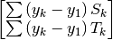
[errata-reei-4]

The original expression for $\sigma_1$ in (8) was:

(64)¶ $\sigma_1 = -\frac{1}{B_1} \sqrt{\frac{2}{\pi}}$

The correction is due to the error in the equations (3) and (2)[errata-reei-2]. Notice that $\mu_1$ is unaffected by the change in factor since it is a ratio.

[errata-reei-5]

An extension of [errata-reei-3] to the summary section. The right-most matrix had $y_k - y_1$ replaced with $f_k - f_1$ .

[errata-reei-6]

An extension of [errata-reei-2] to the summary section. The formula for $\sigma_1$ has been corrected.

[errata-reei-7]

The original paper lists equation [9]. There is no equation [9] in the paper, and contextually, it makes sense that the reference is in fact to equation [1].

[errata-reei-8]

The equation numbers have been moved back by two. The number in the appendix of the original paper starts with 11. However, numbers 9 and 10 are missing from the last numbered equation (which was (8)). There are four unlabeled equations in Appendix 1, not 2.

[errata-reei-9]

The table was extracted from the original figure and added as a separate entity. A caption was added to reflect the caption of Table 1.

[errata-reei-10]

The figure is listed as 11 in the original paper. I am pretty sure that is an outright typo.

[errata-reei-11]

The original paper has the figure number listed as 1 here, but should be 2.

[errata-reei-12]

The equation was moved to a separate line, for consistency with all the other numbered equations in the paper.

[errata-reei-13]

The version of (50) in the original paper has an unbalanced closing parenthesis after $D$ . It has been removed in the translation.

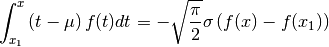
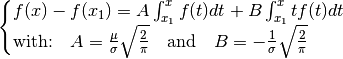
[errata-reei-14]

It is a bit unclear as to how the $f'_k$ values were generated in the figure in the original paper. The x-values of the points appear to be half way between the exact x-values. This makes it reasonable to suppose that the values were calculated from $(x_k, y_k)$ with something like $f'_k = \frac{y_{k+1} - y_k}{x_{k+1} - x_k}$ for $k$ from $1$ to $n-1$ . This is the black line in the generated plot, but it does not match the original figure at all. Using the first equation in 2. Principle of Linearization Through Differential and/or Integral Equations (describing $D_k$ ) does not help either in this case.

[errata-reei-15]

The figure shown here is generates identical results to the one in the original paper, but it is not strictly correct. For each value of $n_p$ , the following code generates the $x$ and $y$ values used to compute $\omega_1$ :

omega_e = 2.0 * np.pi
x = np.linspace(0.0, 1.0, p)
y = np.sin(omega_e * x)

This is not quite correct. The actual x-values should be generated with np.linspace(0.0, 1.0, p, endpoint=False). Put another way, the data in the paper appears to be generated for values of $n_p - 1$ rather than $n_p$ . The overall point being made holds regardless, of course.

[errata-reei-16]

The original figure shows the “exact” $\theta$ line slightly elevated above the “exact” $\Phi$ line, so as not to obscure the portion of $\Phi$ where they match. I have chosen instead to match the lines but make the dotted line thicker, so it is not completely obscured.

[errata-reei-17]

The original list of points was written as $(x_1, t_1, ...; y_1), (x_2, t_2, ...; y_2), ..., (x_k, t_k, ...; y_j), ..., (x_n, t_n, ...; y_m)$ . This implies that the indices of dependent values, $y$ , are not in lockstep with the independent parameters $x, t, ...$ , which is misleading. It is also inconsistent with the subsequent exposition. I have therefore taken the liberty of using the same index for the dependent variables as for the independent.