REGRESSIONS et EQUATIONS INTEGRALES
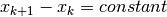
Jean Jacquelin
[ First Edition : 14 January 2009 - Updated : 3 January 2014 ]
Translator’s Note
I came across this paper while searching for efficient, preferably non-iterative, routines for fitting exponentials. The techniques presented in this paper have served my purpose well, and this translation (and to some extent the entire scikit) were the result. I hope that my endeavors do justice to Jean Jacquelin’s work, and prove as useful to someone else as they did to me.
The paper translated here is a compilation of related original papers by the author, gathered into a single multi-chapter unit. Some of the original material is in French and some in English. I have attempted to translate the French as faithfully as I could. I have also attempted to conform the English portions to what I consider to be modern American usage.
There are certain to be some imperfections and probably outright errors in the translation. The translation is not meant to be a monolith. It is presented on GitLab so that readers so inclined can easily submit corrections and improvements.
A small number of technical corrections were made to the content of this paper throughout the translation. In all cases, the errata are clearly marked with footnotes with detailed descriptions of the fix in question. Errata are to be submitted to Jean Jacquelin before publication of this translation.
I have re-generated the plots and tables in the paper as faithfully as I could, rather than copying them out of the original. This has provided a measure of confidence in the results. There may be some slight disagreement in the randomly generated datasets, but the discrepancies are both expected and miniscule.
- – Joseph Fox-Rabinovitz
- 23rd September 2018
Regressions and Integral Equations
Jean Jacquelin
Abstract
The primary aim of this publication is to draw attention to a rarely used method for solving certain types of non-linear regression problems.
The key to the method presented in this paper is the principle of linearization through differential and integral equations, which enables the conversion of a complex non-linear problem into simple linear regression.
The calculus shown shown here has a fundamental difference from traditional solutions to similar problems in that it is non-recursive, and therefore does not require the usual iterative approach.
In order to demonstrate the theory through concrete application, detailed numerical examples have been worked out. Regressions of power, exponential, and logarithmic functions are presented, along with the Gaussian and Weibull distributions commonly found in statistical applications.
Regressions and Integral Equations
Jean Jacquelin
1. Introduction
The study presented here falls into the general framework of regression
problems. For example, given the coordinates of a sequence of  points:
 , we wish to
find the function
, we wish to
find the function 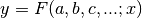 which lies as close as
possible to the data by optimizing the parameters
which lies as close as
possible to the data by optimizing the parameters 
The commonly known solution to linear regression merits only a brief discussion, which is to be found in Appendix 1. Some problems can be solved through linear regression even though they appear non-linear at first glance. The Gaussian cumulative distribution function is a specific example which is discussed in Appendix 2.
Excepting such simple cases, we are confronted with the daunting problem of non-linear regression. There is extensive literature on the subject. Even the most cursort review would derail us from the purpose of this paper. It is also unnecessary because our goal is to reduce non-linear problems to linear regression through non-iterative and non-recursive procedures (otherwise, how would our proposed method be innovative with respect to existing methods?).
In the next section, we will proceed to the heart of the matter: rendering non-linear problems to linear form by means of suitable differential and/or integral equations. The preliminary discussion will show that in the context of such problems, integral equations tend to be more numerically stable than differential equations, with very few exceptions.
The principle of using integral equations will be explained and demonstrated in practice using the Gaussian probability distribution function as a concrete example. Other examples of regression using integral equations will be described in a detailed manner in the two following papers:
2. Principle of Linearization Through Differential and/or Integral Equations
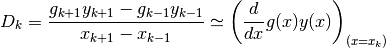
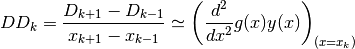
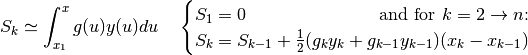
We begin with a summary of numerical methods for approximating derivatives and
integrals. Given points  located near the curve of
a function
located near the curve of
a function  , and given another function
  , we can
calculate approximations for the following derivatives and integrals with
, we can
calculate approximations for the following derivatives and integrals with
 :
:
And so on, for subsequent derivatives, as necessary.
And do on, for subsequent integrals, as necessary.

It goes without saying that the points must first be ranked in order of
ascending  .
.
It is possible to use more sophisticated approximations for numerical
differentiation and integration. Nothing prevents us from selecting a lower
limit (or lower limits) of integration other than  , and using
different limits for the successive integrations. However, that would
complicate the formulas and explanations unnecessarily. For the sake of
simplicity, let us agree to use these formulas, at least for this stage of the
presentation.
, and using
different limits for the successive integrations. However, that would
complicate the formulas and explanations unnecessarily. For the sake of
simplicity, let us agree to use these formulas, at least for this stage of the
presentation.
Returning to our initial formulation of the problem, we wish to optimize the
parameters of a function  so
that its curve approaches the points as closely as
possible. Evidently, the exact expressions of the derivatives and
anti-derivatives of the function depend on the pameters .
However the approximate values calculated using the formulas shown above, i.e.
the numerical values of
so
that its curve approaches the points as closely as
possible. Evidently, the exact expressions of the derivatives and
anti-derivatives of the function depend on the pameters .
However the approximate values calculated using the formulas shown above, i.e.
the numerical values of  , are computed
solely from the data points
, are computed
solely from the data points  , without requiring prior
knowledge of . This observation is the crux of the method
that is to be shown.
, without requiring prior
knowledge of . This observation is the crux of the method
that is to be shown.
Let us suppose that the function is the solution to
a differential and/or integral equation of the form:

with  predetermined functions
independent of , and
predetermined functions
independent of , and
 dependent on . The
approximate values are then respectively (with
dependent on . The
approximate values are then respectively (with
 )[errata-reei-1]:


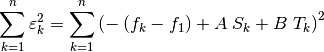
If we replace the exact derivatives and/or anti-derivatives with their numerical approximations, the equation will no longer hold true. We can therefore work with the sum of the squares of the residuals:

The relationship is linear with respect to
. We have therefore returned to
classical linear regression, which allows us to calculate the optimal values of
 . Finally, since
are known functions of
, we must solve the system of equations
. Finally, since
are known functions of
, we must solve the system of equations
 to obtain the optimal values of the parameters .
There are some additional considerations that must be taken into account when
choosing the differental and/or integral equation. Other than the requirement
for linearity in its coefficients (but not necessarily in the functions, since
we have the choice of  ), the equation
should preferably have as many coefficients
), the equation
should preferably have as many coefficients
 as there are initial parameters
to optimize. If there are fewer coefficients, an
additional regression (or regressions) will be necessary to calculate the
coefficients that do not figure explicitly in the equation.
as there are initial parameters
to optimize. If there are fewer coefficients, an
additional regression (or regressions) will be necessary to calculate the
coefficients that do not figure explicitly in the equation.
Moreover, to avoid an overburdened explanation, we have been considering a
simplified form of differential and/or integral equation. In fact, the equation
could have any number of different functions  , several different
derivatives (corresponding to various choices of ), several
different integrals (corresponding to various choice of
, several different
derivatives (corresponding to various choices of ), several
different integrals (corresponding to various choice of  ), and so
on for subsequent multiple derivatives and integrals.
), and so
on for subsequent multiple derivatives and integrals.
Clearly, there is a multitude of choices for the differential and/or integral
equation that we bring to bear on the problem. However, practical
considerations limit our choices. One of the main stumbling blocks is the
difficulty inherent in numerical approximation of derivatives. In fact, in
cases where the points have an irregular distribution, and are too sparse, and
if, to make matters worse, the values of  are not sufficiently
precise, the computed derivatives will fluctuate so much and be so dispersed as
to render the regression ineffective. On the other hand, numerical
approximations of integrals retain their stability even in these difficult
cases (this does not mean that the inevitable deviations are insignificant, but
that they remain damped, which is essential for the robustness of the overall
process). Except in special cases, the preference is therefore to seek an
integral equation rather than a differential one.
are not sufficiently
precise, the computed derivatives will fluctuate so much and be so dispersed as
to render the regression ineffective. On the other hand, numerical
approximations of integrals retain their stability even in these difficult
cases (this does not mean that the inevitable deviations are insignificant, but
that they remain damped, which is essential for the robustness of the overall
process). Except in special cases, the preference is therefore to seek an
integral equation rather than a differential one.
The generality of the presentation that has just been made may give the impression that the method is complicated and difficult to implement in practice. The fact of the matter is quite the opposite, as we will see once we shift focus from an the abstract discussion of many possibilities to solving a single concrete example.
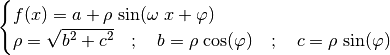
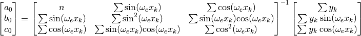
One of the most spectacular examples is that of sinusoidal regression (which
we only mention in passing, without going into depth here, but which will be
treated in detail in the attached paper Regression of Sinusoids). It concerns the
optimization of the parameters  and
and  in the
equation:
in the
equation:

This function is the solution to the differential equation:
This is a linear equation with respect to  and
and  , which are
themselves (very simple) functions of
, which are
themselves (very simple) functions of  and . Moreover,
the parameters
and . Moreover,
the parameters  and
and  no longer figure in the differential
equation directly. This case is therefore a typical application of the method,
and among the easiest to implement, except that it contains a second
derivative, which makes it virtually useless. Fortunately, there is no a-priori
reason not to use an integral equation whose solution is a sinusoid instead.
The integral method is hardly any more complicated and gives largely
satisfactory results (which are studied in detail in the attached paper:
Regression of Sinusoids).
no longer figure in the differential
equation directly. This case is therefore a typical application of the method,
and among the easiest to implement, except that it contains a second
derivative, which makes it virtually useless. Fortunately, there is no a-priori
reason not to use an integral equation whose solution is a sinusoid instead.
The integral method is hardly any more complicated and gives largely
satisfactory results (which are studied in detail in the attached paper:
Regression of Sinusoids).
For our first demonstration of the method, let us look for a simpler example. In the following section, the method of regression through an integral equation will be applied to the Gaussian probability density function.
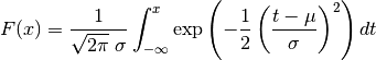
3. Example: Illustration of the Gaussian Probability Density Function
We consider a probability density function of two parameters,  and
and  , defined by
(1)
The general notation of the previous sections is replaced with
 here due to the specificity of this case.
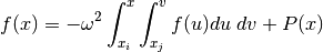
The integration (2) leads to the integral equation
(3), of which is the solution[errata-reei-2]:
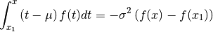
This is a linear integral equation, consisting of two simple integrals, which
places it among the applications mentioned in the previous section. We compute
the respective approximations, the first denoted  with
with
 , and the second denoted
  with
with  :
:
When we replace  with
with  ,
,  with
with
 and the integrals with
  and
and  , respectively,
equation (3) no longer holds true. We seek to minimize the sum of
the squares of the residuals:
, respectively,
equation (3) no longer holds true. We seek to minimize the sum of
the squares of the residuals:
(6)
Notice that had we chosen a lower limit of integration different from
, it would have changed not only the value of , but also
the numerical values of and , in a way that would cancel
out the differences without changing the final result.
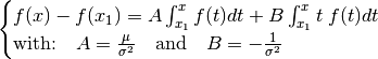
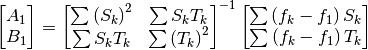
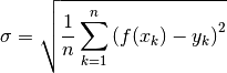
The relationship (6) is none other than the than the equation
of a linear regression, which we know how to optimize for the parameters
 and
and  [errata-reei-3]:
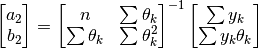
(7)
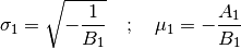
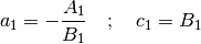
By convention,  . We then deduce
 and
and  according to (3)[errata-reei-4]:
(8)
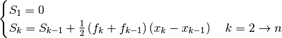
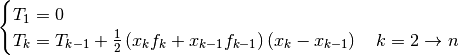
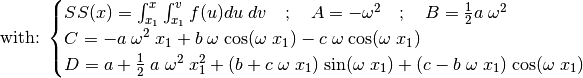
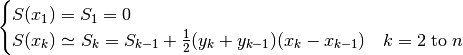
Here is a summary of the numerical computation:
Data:
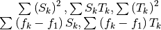
Compute
Compute
Compute
Compute
Compute
Result:

To illustrate the calculation (Fig. 1), numerical data
(Table 1) was genererated in the following manner:
values were chosen at random from the domain under consideration.
From the “exact” values  and
and  (defining the
“exact” function , whose representative curve is plotted as a
dashed line in Fig. 1), we computed the exact values of
given by equation (1)[errata-reei-7]. We then
added perturbations whose amplitude was drawn randomly from a range - to +10%
of , which, after rounding, gave us the numerical values of
in Table 1.
(defining the
“exact” function , whose representative curve is plotted as a
dashed line in Fig. 1), we computed the exact values of
given by equation (1)[errata-reei-7]. We then
added perturbations whose amplitude was drawn randomly from a range - to +10%
of , which, after rounding, gave us the numerical values of
in Table 1.
The outrageous error model is motivated by the need for legibility in the figure, so that the so called “experimental” points, represented by crosses, lie far enough from the dashed curve to be clearly distinguishable. In the same vein, only a handful of points was chosen so that the deviations between the “exact” dashed curves and the calculated solid curves are are highlighted for both the intermediate and the final calculation. The fact that the points are not uniformly distributed across the domain is also a significant complication.
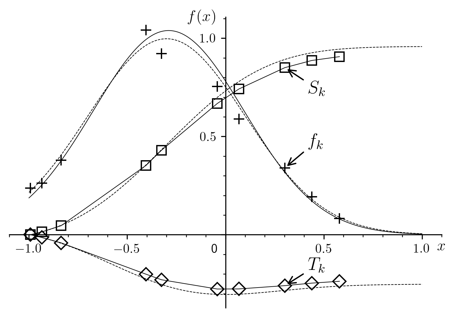
Fig. 1 A sample regression of the Gaussian probability density function.
 |
|
|
|
|
|
|---|---|---|---|---|---|
| 1 | -0.992 | 0.238 | 0 | 0 | |
| 2 | -0.935 | 0.262 | 0.01425 | -0.0137104 | = 0.4 |
| 3 | -0.836 | 0.38 | 0.046029 | -0.0415616 | = -0.3 |
| 4 | -0.404 | 1.04 | 0.352965 | -0.201022 | |
| 5 | -0.326 | 0.922 | 0.429522 | -0.229147 | = 0.383915 |
| 6 | -0.042 | 0.755 | 0.667656 | -0.276331 | = -0.289356 |
| 7 | 0.068 | 0.589 | 0.741576 | -0.275872 | |
| 8 | 0.302 | 0.34 | 0.850269 | -0.259172 | |
| 9 | 0.439 | 0.193 | 0.88678 | -0.246335 | |
| 10 | 0.58 | 0.083 | 0.906238 | -0.236968 |
In Fig. 1, the shape of the curves of the “exact”
integrals and the points  and
and
 make the primary reason for the deviations in
this method of calculation clearly apparent: numerical integration, while
preferable to derivation, is not by any means perfect, and causes the
deviations in
make the primary reason for the deviations in
this method of calculation clearly apparent: numerical integration, while
preferable to derivation, is not by any means perfect, and causes the
deviations in  .
.
To form an objective opinion about the qualities and defects of the method exposed here, it would be necessary to perform a systematic experimental study of a very large number of cases and examples. In the current state of progress of this study, this remains yet to be done.
It is certain that the deviations, caused by the defects inherent in numerical integration, would be considerably reduced if the points were sufficiently numerous and their abscissae were partitioned at sufficiently regular intervals.
4. Discussion
It would be unreasonable to imagine that the method presented here could replace what is currently in use in commercial software, which has the benefits of long term study, experimentation and improvements. We must ask then, what is the motivation behind this work.
Of course, recursive methods generally require a first approximation within the same order of magnitude as the target value. This is not generally a handicap since users are not completely in the dark. One might be tempted to consider this method of integral equations to satisfy the need for initial approximation. However, the need is quite marginal, and should not be seen as a serious motivation.
A simple method, easy to program, like the one shown here, might certainly seduce some potential users in particular situations where we seek full mastery over the calculations that are performed. Users of commercial software are usually satisfied with the results they provide, but may occasionally deplore not knowing precisely what the sophisticated software is doing. Nevertheless, it would be poor motivation indeed for this study to attempt to provide a less powerful tool than what already exists, just to aleviate some of the frustration caused by using tools whose exact mechanisms are unknown.
In fact, we must see in this paper not a specific utilitarian motivation in the case of the Gaussian distribution, but the intention to understand and draw attention to a more general idea: the numerous possibilities offered by integral equations to transform a problem of non-linear regression into a linear regression, computed through a non-iterative process.
It is out of the question to compete against what already exists, and what is more imporant, works well. On the other hand, it would be a pity to forget a method that might potentially help resolve future problems: the method that has been the subject of this paper, whose essence is presented in Section 2.
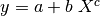
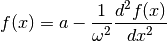
Appendix 1: Review of Linear Regression
When the function that we seek to optimize, , can
be written in the form  ,
according to some number of parameters and with known
functions
,
according to some number of parameters and with known
functions  , the algorithm is linear with respect
to the optimization parameters.
, the algorithm is linear with respect
to the optimization parameters.
Even more generally, if the function can be
transformed into  with known functions
 the algorithm is again linear with respect to the coefficients ,
and
the algorithm is again linear with respect to the coefficients ,
and  , even if it is not linear with respect to
. But it always reverts to a linear regression. The “least
squares” method effectively consists of finding the minimum of:
, even if it is not linear with respect to
. But it always reverts to a linear regression. The “least
squares” method effectively consists of finding the minimum of:
The partial derivatives with respect to  determine a system
of equations for which solutions,
determine a system
of equations for which solutions, 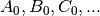 are optimal:
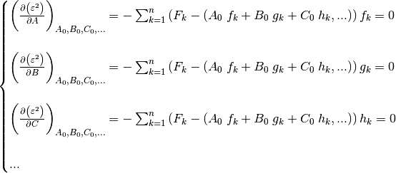
The solution to this system, conventionally written with
leads to:
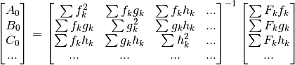
Then we obtain the optimized values of corresponding to
the following system, where the unknowns are  :
:
which is a system that is non-linear in the same measure that the functions
 are non-linear.
But this does not prevent the regression that was performed from being linear,
so even this case has its rightful place in this section.
are non-linear.
But this does not prevent the regression that was performed from being linear,
so even this case has its rightful place in this section.
Of course, this can be further extended by considering more variables, for
example  , instead of just
  , thus working in
3D, or 4D, …, instead of 2D. Everything mentioned here figures in literature
in a more detailed and more structured manner, with presentations adapted to
the exposition of general theory. The purpose here was only to present a brief
review, with a specific notation to be used consistently throughout the
remainder of the work.
, thus working in
3D, or 4D, …, instead of 2D. Everything mentioned here figures in literature
in a more detailed and more structured manner, with presentations adapted to
the exposition of general theory. The purpose here was only to present a brief
review, with a specific notation to be used consistently throughout the
remainder of the work.
Appendix 2: Linear Regression of the Gaussian Cumulative Distribution Function
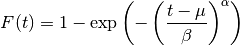
We consider the cumulative Gaussian distribution function of two parameters,
and , defined by[errata-reei-8]:
(9)
An example is shown in Fig. 2 (the dashed curve).
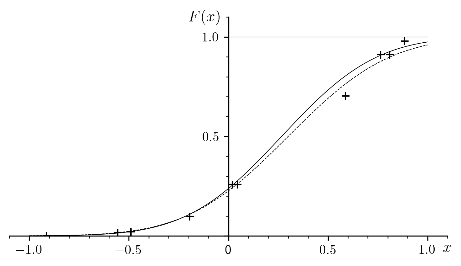
Fig. 2 Sample regression of the Gaussian cumulative distribution function.
|
|
 |
 |
|
|---|---|---|---|---|
| 1 | -0.914 | 0.001 | -2.18512 | |
| 2 | -0.556 | 0.017 | -1.49912 | = 0.4 |
| 3 | -0.49 | 0.021 | -1.43792 | = 0.3 |
| 4 | -0.195 | 0.097 | -0.918416 | |
| 5 | 0.019 | 0.258 | -0.459283 | = 0.374462 |
| 6 | 0.045 | 0.258 | -0.459283 | = 0.266843 |
| 7 | 0.587 | 0.704 | 0.378967 | |
| 8 | 0.764 | 0.911 | 0.952429 | |
| 9 | 0.81 | 0.911 | 0.952429 | |
| 10 | 0.884 | 0.979 | 1.43792 |
The data are the points that we call “experimental”:
 , which, in
Fig. 2[errata-reei-10] have a particular dispersion
relative to their respective nominal positions
, which, in
Fig. 2[errata-reei-10] have a particular dispersion
relative to their respective nominal positions  on the dashed curve representing
  .
.
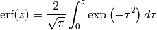
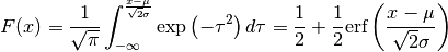
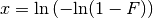
We can write equivalently in terms of the Erf funcion, pronounced
“error function” and defined by:
(10)
The change of variable 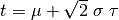 in
(9) gives the relationship:
in
(9) gives the relationship:
(11)
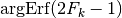
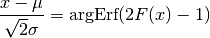
The inverse function to Erf is designated Erf(-1), or Erfinv or argErf. We will use the last notation.
Thus, the inverse relationship to (11) can be written:
(12)
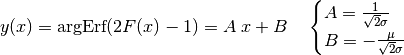
Which in turn leads to a linear relationship in and ,
defined by:
(13)
This reduces to the most elementary form of linear regression, relative to the
points with previously calculated from:
(14)
The optimal values of and are the solutions to the
following system:
(15)
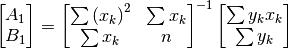
with the convention that . We then deduce
and from (13):
(16)
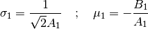
For the example shown, the numerical values of and
that we obtain are shown in Table 2[errata-reei-9].
The curve of the corresponding function is marked with a solid line in
Fig. 2 [errata-reei-11]. It neighbors the “theoretical”
curve, which is dashed.
In fact, the example was intentionally chosen to have a very small number of widely dispersed points, so as to make the two curves clearly distinct from each other. This is depreciative rather than representative of the quality of fit that can usually be obtained.
Here is a summary of the very simple numerical computation:
Data:
Compute
Compute
,
,
,
Compute
Compute
Result:

If a software package implementing argErf is not readily available, a sample listing for the functions Erf and argErf is shown in the next section.
Note: The material in Appendices 1 and 2 is well known. All the same, it was useful to highlight the fundamental differences between the regression problems reviewed in Appendix 1 and those in Section 2 of the main paper. It is equally useful to provide examples that showcase the noteworthy differences between the application of regression to the Gaussian distribution, on one hand to the cumulative function (Appendix 2) and on the other to the more difficult case of the density function (Section 3 of the main text).
Listings for the functions Erf and argErf
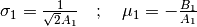
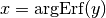
The approximate values of Erf(x) are obtained with a minimum of eight significant digits of precision. We use the following series expansion:
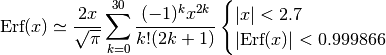
completed by the asymptotic expansion:
The inverse function  is calculated using
Newton-Raphson’s method. The result is obtained to at least eight significant
digits of precision if
is calculated using
Newton-Raphson’s method. The result is obtained to at least eight significant
digits of precision if
 .
Outside that domain, the result is insignificant.
.
Outside that domain, the result is insignificant.
The following listing is written in Pascal, and uses only the most elementary contructs and syntax. It should not be difficult to translate into any other language of choice.
Function Erf(x:extended):extended;
var
   y,p:extended;
   k:integer;
begin
     y:=0;
     p:=1;
     if ((x>-2.7)and(x<2.7)) then
     begin
          for k:=0 to 30 do
          begin
               y:=y+p/(2*k+1);
               p:=-p*x*x/(k+1);
          end;
          y:=y*2*x/sqrt(pi);
     end else
     begin
          for k:= 0 to 5 do
          begin
               y:=y+p;
               p:=-p*(2*k+1)/(2*x*x);
          end;
          y:=y*exp(-x*x)/(x*sqrt(pi));
          if x>0 then y:=1-y else y:=-1-y;
     end;
     Erf:=y;
end;
Function argErf(y:extended):extended;
var
   x:extended;
   k:integer;
begin
     x:=0;
     for k:=1 to 30 do
     begin
          x:=x+exp(x*x)*sqrt(pi)*(y-Erf(x))/2;
     end;
     argErf:=x;
end;
We can test the computation by comparing against the values in the table below (as well as the negatives of the same values):
 |
 |
|---|---|
| 0.001 | 0.001128378791 |
| 0.1 | 0.112462916 |
| 1 | 0.8427007929 |
| 2 | 0.995322265 |
| 2.699 | 0.9998648953 |
| 2.701 | 0.998664351 |
| 4 | 0.9999999846 |
| 5 | 0.9999999999984 |
Non-Linear Regression of the Types: Power, Exponential, Logarithmic, Weibull
Jean Jacquelin
Abstract
The parameters of power, exponential, logarithmic and Weibull functions are optimized by a non-iterative regression method based on an appropriate integral equation.
Non-Linear Regression of the Types: Power, Exponential, Logarithmic, Weibull
Jean Jacquelin
1. Introduction
The following two examples of regression will be treated simultaneously:
Indeed, if we take formula (17), with data points
 , we can pre-calculate
(19)

which turns into (18) with the data points
 .
.
Various other equations can be transformed into these two formulae:
The equation
 is identical to
(18) with the substitution
is identical to
(18) with the substitution  .
.The equation
 turns into
(18) when we interchange the
turns into
(18) when we interchange the  and
and  values. This
motivates the regression of logarithmic functions of three parameters.
values. This
motivates the regression of logarithmic functions of three parameters.Todo
Add to scikit
And so on. In particular, the case of the Weibull function of three parameters will be treated in Section 3.
The method to be used was described in Section 2 of the article Regressions and Integral Equations.
2. Regression of Functions of the Form 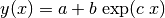 
Integating the function results in:
(20)
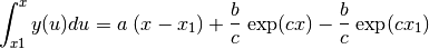
Replacing  with (18):
(21)
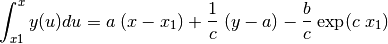
From which we have the integral equation to be used:
(22)
The numerical approximations of the integral for  are calculated
with:
are calculated
with:
(23)
When we replace the exact unknowns in (22) with their respective approxmations, the equation no longer holds true:
(24)

Minimizing the sum of the squared residuals:
(25)
with
(26)

results in a linear regression with respect to the coefficients and
, whose optimal values and can be obtained in
the usual manner (with the convention that ):
(27)

We the get the optimal values  and
and  according to
(26):
according to
(26):
(28)
Only two parameters are resolvable from the form of integral equation that we
chose. The third parameter appears in the numerical calculations, but not
directly in the equation, so another regression is necessary to obtain it. In
fact, considering (18), the result would be further improved by
computing the regression on both and :
(29)
Setting:
(30)

the resulting regression is:
(31)
Here is a summary of the computation:


 , compute
To illustrate this calculation (Fig. 3), numerical data were
generated in the following manner: were drawn at random from the
domain under consideration. Initially, “exact” values  ,
,  and
and  defined the function , which we call the “true”
form of equation (18), and whose curve is traced by a dotted line in
the figure. The exact values of
defined the function , which we call the “true”
form of equation (18), and whose curve is traced by a dotted line in
the figure. The exact values of  were then assigned perturbations
of an amplitude drawn at random from a range between - and +10% of
, which, after rounding, produced the numrical values of
in Table 3, represented by crosses in the figure.
were then assigned perturbations
of an amplitude drawn at random from a range between - and +10% of
, which, after rounding, produced the numrical values of
in Table 3, represented by crosses in the figure.
Finally, the result  was substituted into equation
(18), to obtain the fitted curve, plotted as a solid line.
was substituted into equation
(18), to obtain the fitted curve, plotted as a solid line.
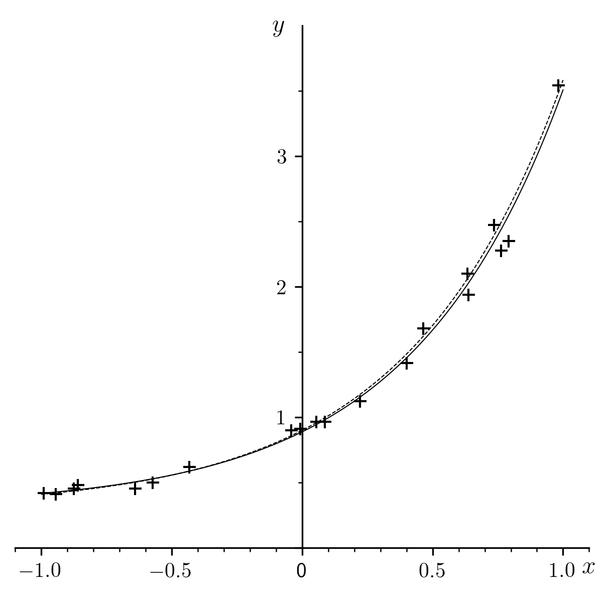
Fig. 3 A sample regression for the function 
|
|
|
|
|
|---|---|---|---|---|
| 1 | -0.99 | 0.418 | 0 | |
| 2 | -0.945 | 0.412 | 0.018675 | = 0.3 |
| 3 | -0.874 | 0.452 | 0.049347 | = 0.6 |
| 4 | -0.859 | 0.48 | 0.056337 | = 1.7 |
| 5 | -0.64 | 0.453 | 0.1585 | |
| 6 | -0.573 | 0.501 | 0.19046 |  = 0.313648 = 0.313648 |
| 7 | -0.433 | 0.619 | 0.268859 |  = 0.574447 = 0.574447 |
| 8 | -0.042 | 0.9 | 0.565824 |  = 1.716029 = 1.716029 |
| 9 | -0.007 | 0.911 | 0.597517 | |
| 10 | 0.054 | 0.966 | 0.654765 | |
| 11 | 0.088 | 0.966 | 0.687609 | |
| 12 | 0.222 | 1.123 | 0.827572 | |
| 13 | 0.401 | 1.414 | 1.05463 | |
| 14 | 0.465 | 1.683 | 1.15374 | |
| 15 | 0.633 | 2.101 | 1.47159 | |
| 16 | 0.637 | 1.94 | 1.47968 | |
| 17 | 0.735 | 2.473 | 1.69591 | |
| 18 | 0.762 | 2.276 | 1.76002 | |
| 19 | 0.791 | 2.352 | 1.82713 | |
| 20 | 0.981 | 3.544 | 2.38725 |
To form an objective opinion of the qualities and defects of the method presented here, it would be necessary to perform a systematic study of a very large number of cases and examples. It is certain even now that the deviations caused by errors in numerical integration would be considerably reduced as the number of points increases and their spacing becomes more uniform.
3. Regression of the Three-Parameter Weibull Cumulative Distribution Function
The Weibull cumulative distribution function of three parameters
( ,
,  , and ) is defined by:
(32)
For data given as  , we seek
to optimize , , and in such a way that
relationship (32) is approximately and optimally satisfied
across the data points.
, we seek
to optimize , , and in such a way that
relationship (32) is approximately and optimally satisfied
across the data points.
The inverse function of (32) is:
(33)
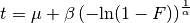
Setting:
(34)
and:
(35)
We can see immediately that we have transformed the problem into (18),
shown above: .
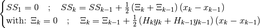
The algorithm is deduced immediately as we transpose the notation:
Data
Procedure
Rank points in order of ascending
Compute
Compute
Compute
Obtain
Compute
Compute
and
:
Result:
,


In graphical representations, it is customary to display  as the abscissa and
  as the ordinate.
This is a legacy of the graphical linearization method used for the case where
as the ordinate.
This is a legacy of the graphical linearization method used for the case where
 . In order to respect this tradition, we will interchange the
axes and display as the abscissa and as the
ordinate.
. In order to respect this tradition, we will interchange the
axes and display as the abscissa and as the
ordinate.
Weibull’s law applies generally to the failure of materials and objects. Since
the variable  is time, the
  and are effectively
sorted in ascending order.
and are effectively
sorted in ascending order.
A sample regression is shown in Fig. 4. To simulate an
experiment, numerical data  were generated from “exact”
values
were generated from “exact”
values  ,
,  , , defining the “true”
 according to (32), whose curve is shown as a
dashed line in the figure. A value of calculated from
(33) corresponds to each . These values of
are subjected to random deviations, simulating experimental
uncertainty, which gives us the values of in
Table 4. Finally, the result (,
, and ) substituted into (32) gives
the “fitted” function
according to (32), whose curve is shown as a
dashed line in the figure. A value of calculated from
(33) corresponds to each . These values of
are subjected to random deviations, simulating experimental
uncertainty, which gives us the values of in
Table 4. Finally, the result (,
, and ) substituted into (32) gives
the “fitted” function  (whose curve is plotted as a solid line):
(36)
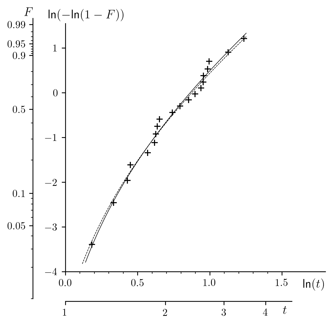
Fig. 4 A sample regression of a Weibull cumulative distribution function of three parameters.
|
|
|
|
|
|
|---|---|---|---|---|---|
| 1 | 1.202 | 0.033 | -3.39452 | 0 | |
| 2 | 1.397 | 0.082 | -2.45856 | 1.21627 | = 2.4 |
| 3 | 1.537 | 0.131 | -1.96317 | 1.94301 | = 1.6 |
| 4 | 1.57 | 0.181 | -1.61108 | 2.48998 | = 0.8 |
| 5 | 1.768 | 0.23 | -1.34184 | 2.93935 | |
| 6 | 1.856 | 0.279 | -1.11744 | 3.34596 | = 2.44301 |
| 7 | 1.87 | 0.328 | -0.922568 | 3.70901 | = 1.55262 |
| 8 | 1.889 | 0.377 | -0.748219 | 4.0367 | = 0.82099 |
| 9 | 1.918 | 0.426 | -0.58856 | 4.3406 | |
| 10 | 2.098 | 0.475 | -0.439502 | 4.63991 | |
| 11 | 2.212 | 0.524 | -0.297951 | 4.94496 | |
| 12 | 2.349 | 0.573 | -0.161377 | 5.25641 | |
| 13 | 2.453 | 0.622 | -0.027514 | 5.57782 | |
| 14 | 2.557 | 0.671 | 0.105888 | 5.91199 | |
| 15 | 2.596 | 0.72 | 0.241349 | 6.26101 | |
| 16 | 2.602 | 0.769 | 0.382086 | 6.62678 | |
| 17 | 2.678 | 0.818 | 0.532831 | 7.02475 | |
| 18 | 2.706 | 0.867 | 0.701813 | 7.47965 | |
| 19 | 3.089 | 0.916 | 0.907023 | 8.07424 | |
| 20 | 3.441 | 0.965 | 1.20968 | 9.06241 |
The representation in the traditional coordinate system shows that the presence
of a non-zero parameter prevents the usual graphical
linearization, which is naturally to be expected. Carrying out the regression
through an integral equation allows us to linearize and obtain a curve which
may be substituted for the traditional method, appreciably improving the fit.
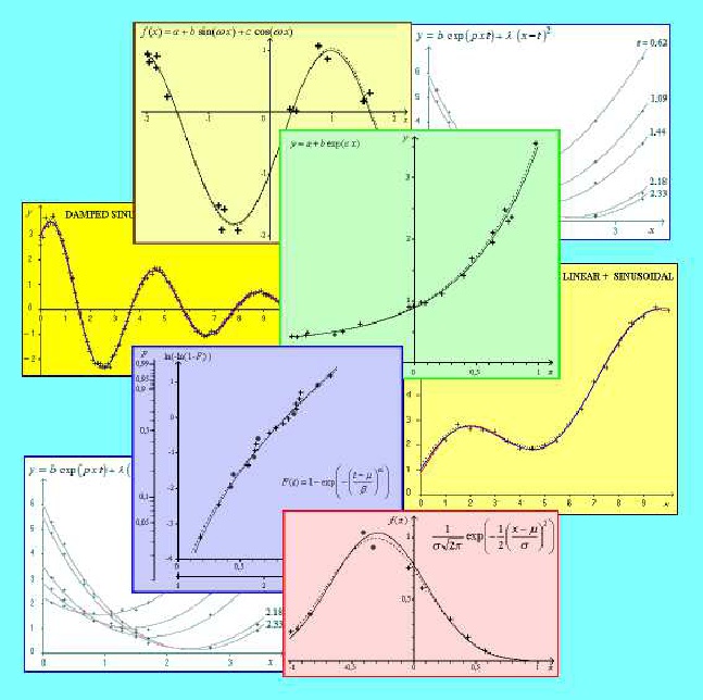
Regression of Sinusoids
Jean Jacquelin
1. Introduction
Under the seemingly innocuous title “Regression of Sinusoids”, ought to appear the subtitle “An Optimization Nightmare” to add a touch of realism. Indeed, we must have already been concerned with the problem to fully understand the relevance of the word. But what is it, really?
As with any number of similar problems, the data is comprised of
experimental points
. We seek to
adjust the parameters of a function  in such a way that its
curve passes “as closely as possible” to the data points. In this particular
case, we will deal with the following sinusoidal function of the four
parameters , , , and :
in such a way that its
curve passes “as closely as possible” to the data points. In this particular
case, we will deal with the following sinusoidal function of the four
parameters , , , and :
(37)
This function is equivalent to:
(38)
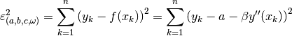
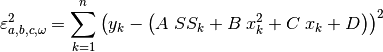
The expression “as closely as possible” implies an optimization criterion. Specifically, we consider the sum of the squared residuals:
(39)
Since that is the sum that we wish to minimize, we have the generic name “least squares method”.
When is known a-priori, the solution is trivial. Equation
(37) effectively becomes linear in the optimization parameters
(, and ). This well defined case merits only the
briefest mention, which will be made in the next section.
In all other cases, the regression (or optimization) is non-linear, due to the
fact that the sum of squares has a non-linear dependency on .
An almost equally favorable situation arises when we have a “good enough”
approximation for , suitable to initialize an arbitrary
non-linear optimization method. Literature is full of descriptions of such
methods and many are implemented in software. To discuss these methods further
would exceed the scope of the framework of this paper.
But the dreaded nightmare is not far. It is crucial that the initial estimate
for is “good enough”… And this is where sinusoidal functions
differ from more accomodating non-linear functions: The more periods that the
span, the more randomly they are distributed, or the more noise is
present in the values, the more the condition “good enough” must be
replaced with “very good”, tending to “with great precision”. In other words,
we must know the value of we are looking for in advance!
The original method proposed in Section 3 provides a
starting point for addressing this challenge. Admittedly, it would be wrong to
pretend that the method is particularly robust: Section 4
will discuss some of its deficiencies. Nevertheless, thanks to the first
result, we will see in Section 5 that an original
regression method (a saw’s tooth), allows for a much more accurate
approximation of through an improved linearization. Finally,
Section 6 presents a summary of preformance in the course
of systematic experiments. A synopsis of the entire method, which does not
involve any iterative calculations, is presented in the
Appendices.
Before getting into the heart of the matter, a warning must be given regarding some of the figures presented here (Fig. 5, Fig. 6, Fig. 7, Fig. 11, Fig. 14). They serve merely as illustrations of the procedures being described. To create them, we were obligated to fix on a particuar numeroical data set, which is not necessarily representative of the multitudes of possible cases. Given these figures alone, it would be absurd to form any opinion of the method in question, favorable or otherwise. This is especially true as the example has been selected with data that exaggerate all the defects that are explained in the text, to allow for easy identification and unambiguous discussion of the important features.
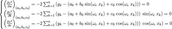
We see in Table 5 that our “experimental” points are
sparse, non-uniformly distributed, and widely dispersed. One might suspect that
this is not real experimental data, but rather a simulation obtained in the
following way: An “exact” function is given, along with the coefficients
, , , and  , indicated in
Table 5. The curve is plotted in
Fig. 5 with a dashed line. The were selected
at random from the domain, and rounded to the values shown in
Table 5. The corresponding exact values are
then computed from equation (37). The were then randomly
perturbed with a distribution whose root mean square was
approximately 10% of the amplitude
, indicated in
Table 5. The curve is plotted in
Fig. 5 with a dashed line. The were selected
at random from the domain, and rounded to the values shown in
Table 5. The corresponding exact values are
then computed from equation (37). The were then randomly
perturbed with a distribution whose root mean square was
approximately 10% of the amplitude  of the sinusoid. This
represents a much wider dispersion compared to what is usually seen in
practice.
of the sinusoid. This
represents a much wider dispersion compared to what is usually seen in
practice.
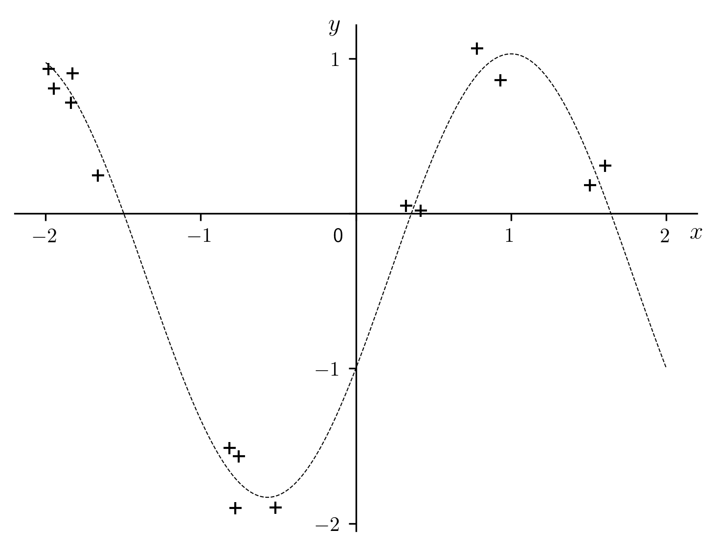
Fig. 5 “Exact” sinusoid along with the numerical data of our example.
|
|
|
|
|---|---|---|---|
| 1 | -1.983 | 0.936 | |
| 2 | -1.948 | 0.810 | = 2 |
| 3 | -1.837 | 0.716 | = -0.4 |
| 4 | -1.827 | 0.906 | = 1.3 |
| 5 | -1.663 | 0.247 | = -0.6 |
| 6 | -0.815 | -1.513 | = 1.431782 |
| 7 | -0.778 | -1.901 | = 0.1491 |
| 8 | -0.754 | -1.565 | |
| 9 | -0.518 | -1.896 | |
| 10 | 0.322 | 0.051 | |
| 11 | 0.418 | 0.021 | |
| 12 | 0.781 | 1.069 | |
| 13 | 0.931 | 0.862 | |
| 14 | 1.510 | 0.183 | |
| 15 | 1.607 | 0.311 |
The root mean square is defined by:
(40)
The values of the function are to be computed using the parameters
, , and from the example under
consideration.
The values of , indicated in Table 5 and
plotted in Fig. 5, are the data for the numerical
examples in the following sections. It should be noted that the exact values
, , and , shown in
Table 5 are not used further on (except
in the “trivial” case in Section 2). They should be
forgotten for the remainder of the algorithm, which uses only
as data. While the exact sinusoid will be shown on the
various figures as a reminder, it is not an indication of the fact that the
function (37) with the parameters ( ) is
ever used directly.
) is
ever used directly.
The tables serve another role, which will be appreciated by readers interested in implementing these techniques in a computer program. If so desired, all of the sample calculations shown here can be reproduced exactly with the data and results reported below. This provides a means to validate and correct a regression program implementing the algorithms described here.
2. Case Where is Known A-Priori
When the value  is fixed, the optimization only needs
to be performed for the parameters , and of
(37). Taking the partial derivatives of (39) with respect to
the optimization parameters result in a system of three equations:
is fixed, the optimization only needs
to be performed for the parameters , and of
(37). Taking the partial derivatives of (39) with respect to
the optimization parameters result in a system of three equations:
(41)
The solution is given in the following system (42), with the
convention that :
(42)
The result is presented in figure Fig. 6. We note that
the root mean square  is practically identical to
in Table 5. This indicates that the
regression did not increase the residuals of the fitted sinusoid relative to
the “exact” one. Obviously, this is too good to always be true. So, after this
brief review, we must tackle the crux of the problem: to compute a sufficiently
accurate approximation for , since it will not be know a-priori
as it was in the preceding example.
is practically identical to
in Table 5. This indicates that the
regression did not increase the residuals of the fitted sinusoid relative to
the “exact” one. Obviously, this is too good to always be true. So, after this
brief review, we must tackle the crux of the problem: to compute a sufficiently
accurate approximation for , since it will not be know a-priori
as it was in the preceding example.
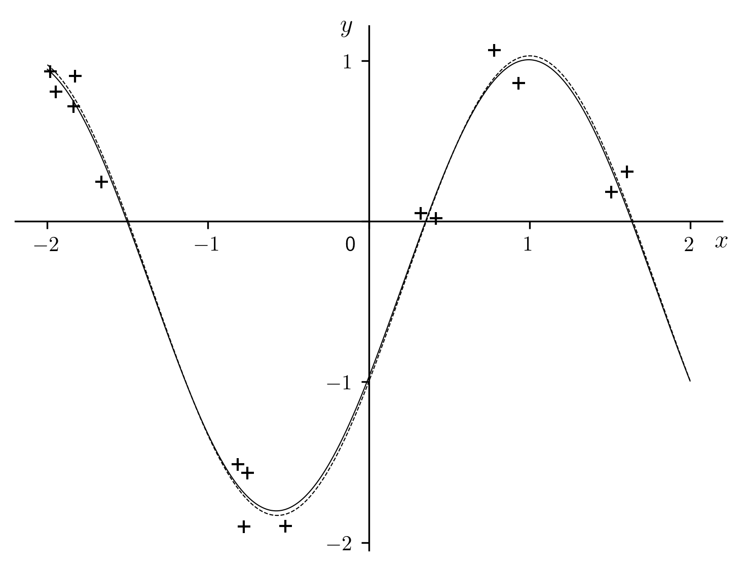
Fig. 6 Case where is know exactly.
| = 2 |
 = -0.397904 = -0.397904 |
 = 1.283059 = 1.283059 |
 = -0.573569 = -0.573569 |
 = 1.405426 = 1.405426 |
| = 0.147456 |
3. Linearization Through an Integral Equation
The goal being to reduce the problem to a linear regression, it is sometimes tempting to use a linear differential equation whose solution is our function of interest as the intermediary. An example is the follwing equation, for which the sinusiod (37) is a solution[errata-reei-12]:
(43)
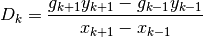
Taking the appropriate partial derivatives of (44) leads to a
system of linear equations of two unknowns and
 .
.
(44)
Unfortunately, this is not a viable solution in practice (unless we have at our
disposal a very large number of especially well distributed samples). The
stumbling block here is the calculation of  from the
data points : as illustrated in Fig. 7,
the fluctuations are generally too unstable for meaningful approximation.
from the
data points : as illustrated in Fig. 7,
the fluctuations are generally too unstable for meaningful approximation.
On the other hand, the computation of numerical integrals is clearly less problematic than that of derivatives. It is therefore no surprise that we will seek an integral equation having for its solution our function of interest. For example, in the present case, we have equation (45), for which the sinusoid (37) is a solution:
(45)
 is a second-degree polynomial whose coefficiens depend on
, , , and the limits of integration
is a second-degree polynomial whose coefficiens depend on
, , , and the limits of integration
 and
and  .
.
We could, of course, go into a great amount of detail regarding ,
but that would derail the presentation without much immediate benefit. We can
simply use the fact that a complete analysis shows that the limits of
integration have no bearing on the regression that follows, at least with
regard to the quantity of interest, the optimized value of
(noted as  ). Therefore, to simplify, we will set
 , which results in a function of the following form:
(46)
(47)
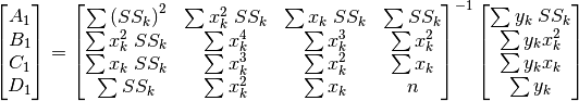
The coefficients , , ,  are unknown.
However, they can be approximated through linear regression based on the
precomputed values of
are unknown.
However, they can be approximated through linear regression based on the
precomputed values of  . To accomplish this, we perform two numeric
integrations:
. To accomplish this, we perform two numeric
integrations:
(48)
(49)
It goes without saying that the points must first be ranked in order of
ascending . It follows that the sum of squared residuals to minimize
is the following[errata-reei-13]:
(50)
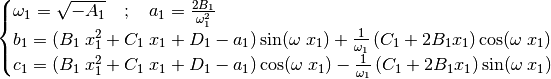
There is no need to reiterate the partial derivatives with respect to
, , and , used to obtain the optimized
, ,  and
and  , followed by ,
 , and (according to
(47)):
, and (according to
(47)):
(51)
(52)
The results for our sample dataset are displayed further along in
Fig. 14. The numerical values of ,
, and are shown in
Table 14. To compare the graphical and numerical
representations with resepect to the data points , refer to
the curve and table column labeled  .
.
Incidentally, it is interesting to compare the results of numerical
integrations (48) and (49) with respect to
differentiation (Fig. 7). Observing the significant
oscillations of the latter (a sample point is noted  on the plot),
and how they would be exacerbated by further differentiation (not shown due to
the excessive fluctuation amplitude), it becomes patently obvious that a
feasible solution must be based on integral equations rather than differential.
on the plot),
and how they would be exacerbated by further differentiation (not shown due to
the excessive fluctuation amplitude), it becomes patently obvious that a
feasible solution must be based on integral equations rather than differential.
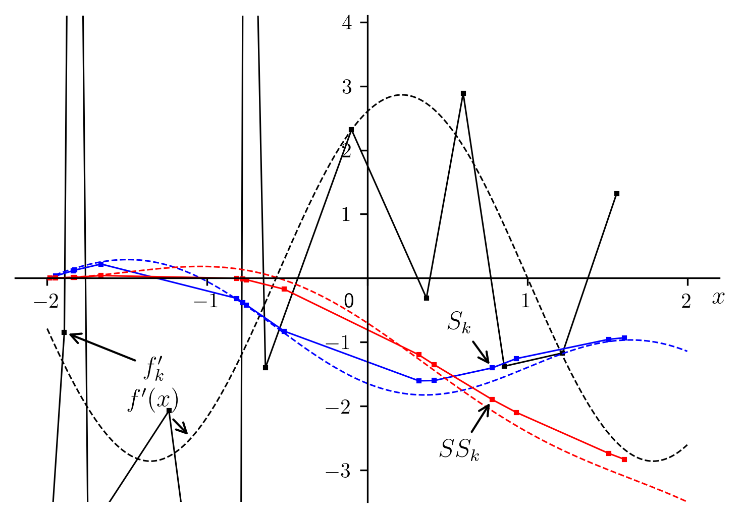
Fig. 7 Numerical integrations and comparison with differentiations.[errata-reei-14].
|
|
|
|---|---|---|
| 1 | 0 | 0 |
| 2 | 0.030555 | 0.000534713 |
| 3 | 0.115248 | 0.00862678 |
| 4 | 0.123358 | 0.00981981 |
| 5 | 0.217904 | 0.0378033 |
| 6 | -0.31888 | -0.00501053 |
| 7 | -0.382039 | -0.0179775 |
| 8 | -0.423631 | -0.0276456 |
| 9 | -0.832029 | -0.175813 |
| 10 | -1.60693 | -1.20018 |
| 11 | -1.60347 | -1.35428 |
| 12 | -1.40564 | -1.90043 |
| 13 | -1.26081 | -2.10041 |
| 14 | -0.958286 | -2.74284 |
| 15 | -0.934327 | -2.83463 |
While noting that with more numerous and uniformly distributed ,
coupled with less scattered would result in more acceptable
fluctuations in the derivatives, we must also remember that a good solution
must apply not only to the trivial cases, but the difficult ones as well.
4. A Brief Analysis of Performance
The most important parameter to optimize is . This comes with the
understanding that once the optimization has succeeded, we can always fall back
to the conventional regression method in Section 2 to
obtain , and . We will therefore concentrate on an
investigation restricted to results with respect to . The three
most influential factors are:
- The number of points,
, in each period of the sinusoid.
- The distribution of samples in the domain:
- Either uniform:
- Or random:
- The scatter of the ordinates
, the ratio of the root mean squared error (40) to the amplitude of the sinusoid.
4.1 Uniform Distribution of Abscissae With Non-Dispersed Ordinates
We find that the ratio  , which is expected to be
equal to 1, is affected by a deviation inversely proportional to
(Fig. 8). It is conceivably possible to construct an
empirical function to correct the deviation. But such a function would not be
very interesting, as the correction would not be satisfactory for the randomly
distributed points we well investigate further on. A more general approach,
described in Section 5, seems more appropriate.
, which is expected to be
equal to 1, is affected by a deviation inversely proportional to
(Fig. 8). It is conceivably possible to construct an
empirical function to correct the deviation. But such a function would not be
very interesting, as the correction would not be satisfactory for the randomly
distributed points we well investigate further on. A more general approach,
described in Section 5, seems more appropriate.
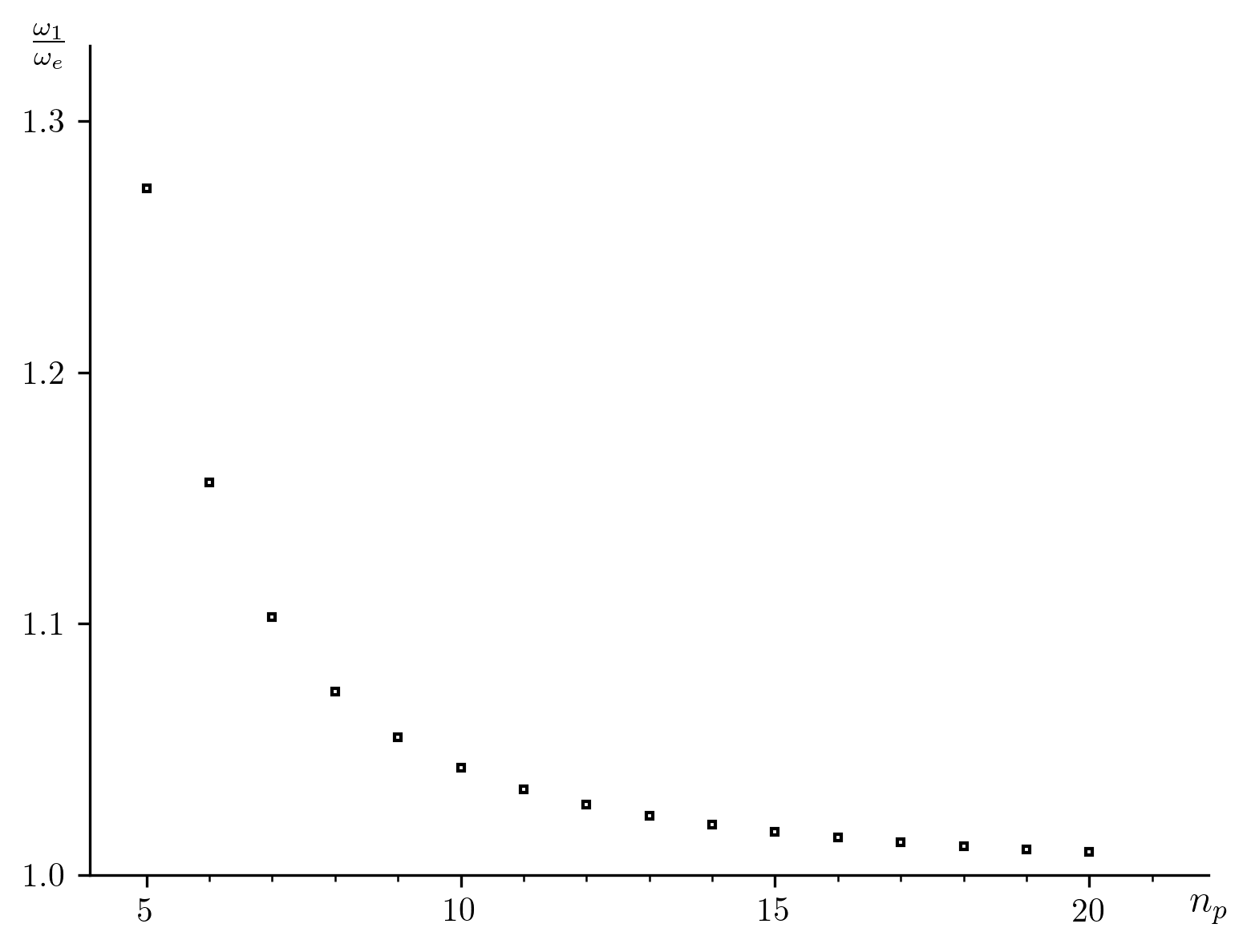
Fig. 8 Effect of the number of points per period, with a uniform distribution.
|
 |
|---|---|
| 5 | 1.273 |
| 6 | 1.156 |
| 7 | 1.103 |
| 8 | 1.073 |
| 9 | 1.055 |
| 10 | 1.043 |
| 11 | 1.034 |
| 12 | 1.028 |
| 13 | 1.023 |
| 14 | 1.02 |
| 15 | 1.017 |
| 16 | 1.015 |
| 17 | 1.013 |
| 18 | 1.012 |
| 19 | 1.01 |
| 20 | 1.009 |
Todo
Place table next to figure if possible: .figure {float: left;}?
4.2 Random Distribution of Abscissae With Non-Dispersed Ordinates
Since are randomly distributed, the dispersion in the calculated
values of increases as becomes small. For a fixed
value of , the cumulative distribution (computed from 10000
simulations), is represented in Fig. 9. It can be seen
that the expected median  , which is expected to be
equal to 1, is affected even more than under the conditions described in
Section 4.1.
, which is expected to be
equal to 1, is affected even more than under the conditions described in
Section 4.1.
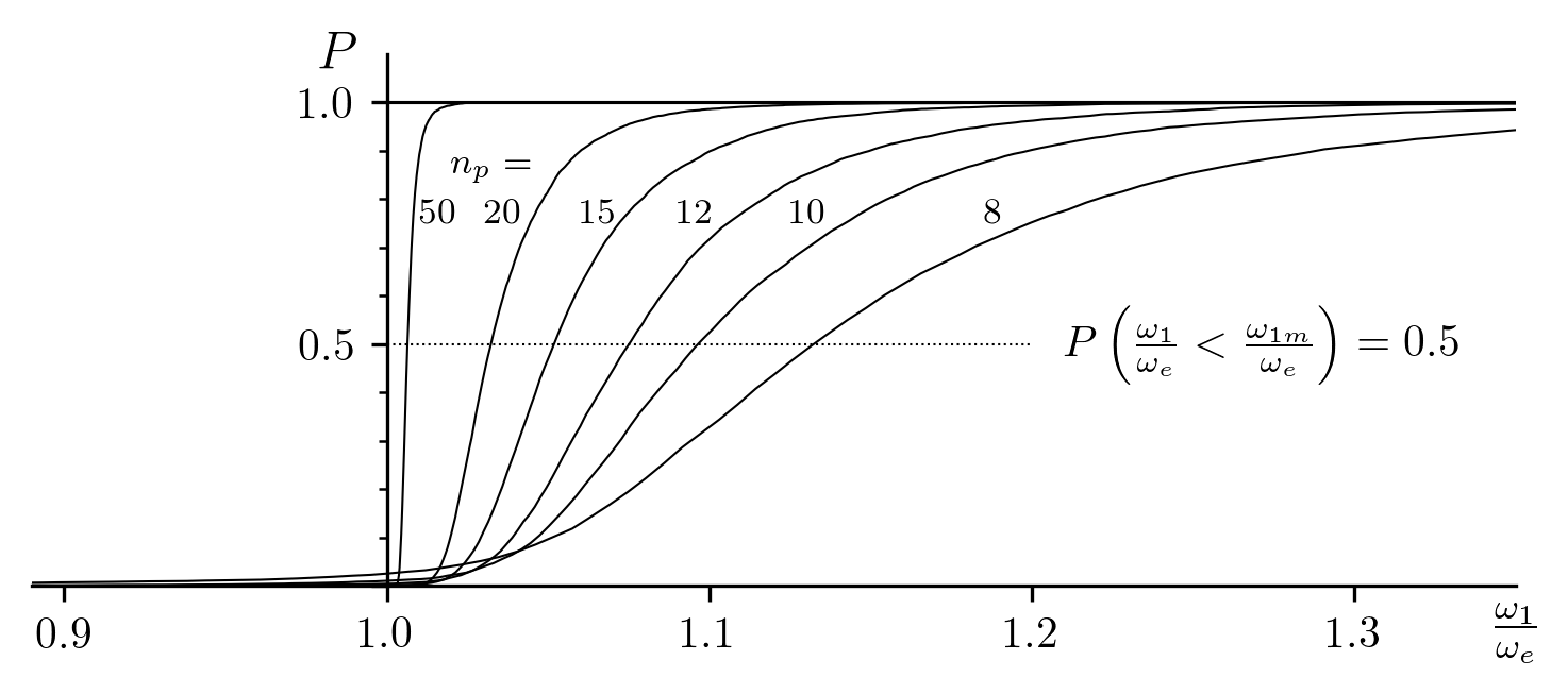
Fig. 9 Cumulative distributions of (random distribution of
, non-dispersed ).
|
 |
|---|---|
| 8 | 1.132 |
| 10 | 1.096 |
| 12 | 1.075 |
| 15 | 1.052 |
| 20 | 1.032 |
| 50 | 1.006 |
Todo
Place table next to figure if possible: .figure {float: left;}?
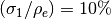
4.3 Random Distribution of Abscissae With Dispersed Ordinates
As expected, the dispersion of is greater than in the previous
case. Fig. 10 shows the the case where
 , compared to
  as
represented in Fig. 9. Nevertheless, the median values
are barely affected (compare Table 10 to the previous
data in Table 9).
as
represented in Fig. 9. Nevertheless, the median values
are barely affected (compare Table 10 to the previous
data in Table 9).
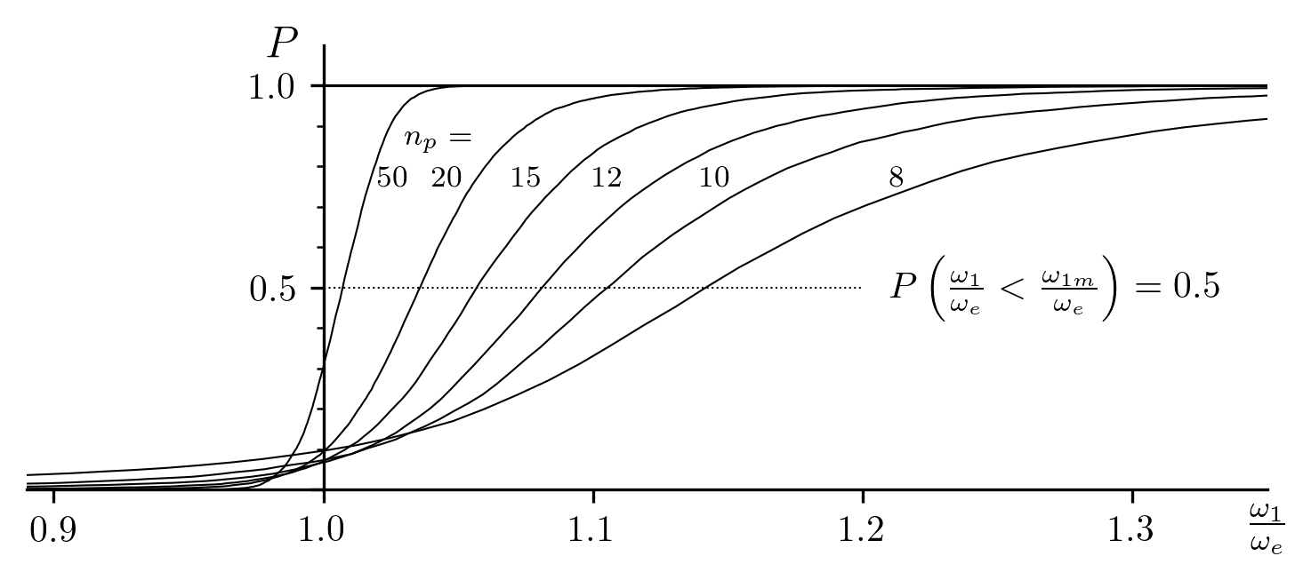
Fig. 10 Cumulative distributions of with randomly distributed ordinates such that 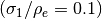
|
|
|---|---|
| 8 | 1.142 |
| 10 | 1.105 |
| 12 | 1.081 |
| 15 | 1.057 |
| 20 | 1.036 |
| 50 | 1.007 |
Todo
Place table next to figure if possible: .figure {float: left;}?
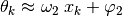
5. Further Optimizations Based on Estimates of and  
We now shift our interest to a function , expressed in the form
(38). The inverse function is an arcsine, but can also be expressed as
an arctangent:
(53)
 denotes the principal values (between
 and
and  ) of the multivalued function.
The sign of
) of the multivalued function.
The sign of  and the integer
  depend on the
half-period of the sinusoid in which the point
depend on the
half-period of the sinusoid in which the point  is found, making
their dependence on discontinuous. Additionally, we can show that the
sign is + when is even and - when odd.
is found, making
their dependence on discontinuous. Additionally, we can show that the
sign is + when is even and - when odd.
If we consider by itself, it is a sawtooth function, as shown
in Fig. 11 by the dotted curve. The points
 , with
  , are represented by
crosses. Rewritten in this manner, the problem becomes one of regression of a
sawtooth function, which is largely as “nightmarish” as regression of the
sinusoid. Since we have no information other than the points
, determining difficult and mostly
empirical, and therefore not guaranteed to always be feasible in the general
case. The situation is different in our case because we have already found the
orders of magnitude of the parameters: , ,
and , and consequently
, are represented by
crosses. Rewritten in this manner, the problem becomes one of regression of a
sawtooth function, which is largely as “nightmarish” as regression of the
sinusoid. Since we have no information other than the points
, determining difficult and mostly
empirical, and therefore not guaranteed to always be feasible in the general
case. The situation is different in our case because we have already found the
orders of magnitude of the parameters: , ,
and , and consequently  and
and  through (38). In the current instance, which will be represented by
the subscript 2, we posit that:
through (38). In the current instance, which will be represented by
the subscript 2, we posit that:
(54)
Now it is possible to calculate  in number
of different ways. One possibility is as follows, where
in number
of different ways. One possibility is as follows, where  rounds the real argument to the nearest integer:
(55)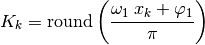
Another way to write (53), applied to , better
demonstrates the nearly linear relationship
 between and
 , defined by:
(56)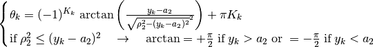
We see in Fig. 11, that the series of points
represented by crosses, is transformed into a series of
points  represented by squares, some of which coincide.
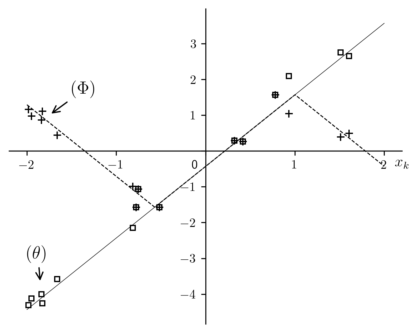
Fig. 11 Transformation of a sawtooth function in preparation for linear regression[errata-reei-16]
|
 |
 |
|
|---|---|---|---|
| 1 | 1.16394 | -1 | -4.30553 |
| 2 | 0.975721 | -1 | -4.11731 |
| 3 | 0.864493 | -1 | -4.00609 |
| 4 | 1.11266 | -1 | -4.25425 |
| 5 | 0.438724 | -1 | -3.58032 |
| 6 | -0.990033 | -1 | -2.15156 |
| 7 | -1.5708 | 0 | -1.5708 |
| 8 | -1.06193 | 0 | -1.06193 |
| 9 | -1.5708 | 0 | -1.5708 |
| 10 | 0.288353 | 0 | 0.288353 |
| 11 | 0.266008 | 0 | 0.266008 |
| 12 | 1.5708 | 1 | 1.5708 |
| 13 | 1.04586 | 1 | 2.09573 |
| 14 | 0.388646 | 1 | 2.75295 |
| 15 | 0.490008 | 1 | 2.65159 |
It is clear that the points tend towards a straight
line, which makes it possible to perform a linear regression to obtain
 from the slope and
  from the x-intercept.
Once we have computed from (56), the result can be
obtained in the usual manner:
from the x-intercept.
Once we have computed from (56), the result can be
obtained in the usual manner:
(57)
Completed by:
(58)
The numerical results are summarized in Table 14 (in the
table column labeled  ), and the curve is shown in
Fig. 14.
), and the curve is shown in
Fig. 14.
The performance measured in terms of the optimization of is
shown in Fig. 12 and Fig. 13.
Note the improvements in the optimized median value,  , shown in
Table 12 and Table 13, which was
the objective of this phase of the algorithm.
, shown in
Table 12 and Table 13, which was
the objective of this phase of the algorithm.
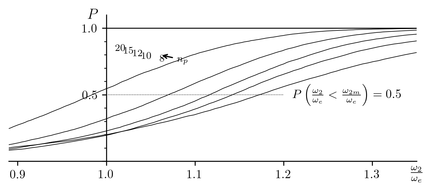
Fig. 12 Cumulative distributions of (random distribution of
, non-dispersed ).
Todo
Fix the broken figure
|
 |
|---|---|
| 8 | 1.173 |
| 10 | 1.142 |
| 12 | 1.117 |
| 15 | 1.070 |
| 20 | 0.984 |
Todo
Fix the broken table
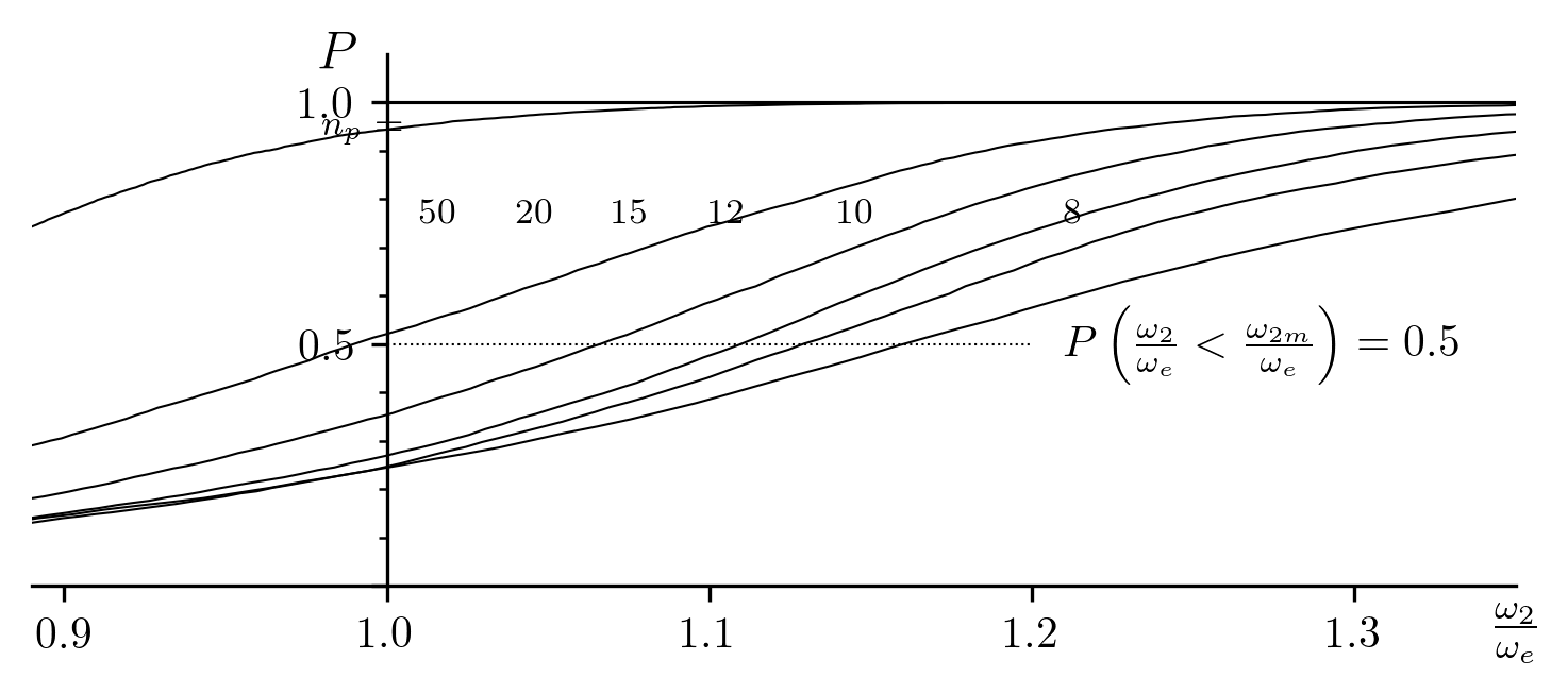
Fig. 13 Cumulative distributions of with randomly distributed ordinates such that 
Todo
Fix the broken figure
|
|
|---|---|
| 8 | 1.160 |
| 10 | 1.129 |
| 12 | 1.110 |
| 15 | 1.066 |
| 20 | 0.990 |
| 50 | 0.825 |
Todo
Fix the broken table
6. Final Steps and Results
As soon as we have a good approximation () of ,
the classical method shown in Section 2 can be applied:
(59)
This allows us to perform a final optimization of the dimensional parameters of
the sinusoid, which was not possible in the previous step because
and  were fixed. The final result is presented in
Fig. 14. The numerical results are summarized in
Table 14 (in the table column labeled
were fixed. The final result is presented in
Fig. 14. The numerical results are summarized in
Table 14 (in the table column labeled  ). The
intermediate results (sinusoids and , along with their
respective parameters) are reported in the same figure and table.
). The
intermediate results (sinusoids and , along with their
respective parameters) are reported in the same figure and table.
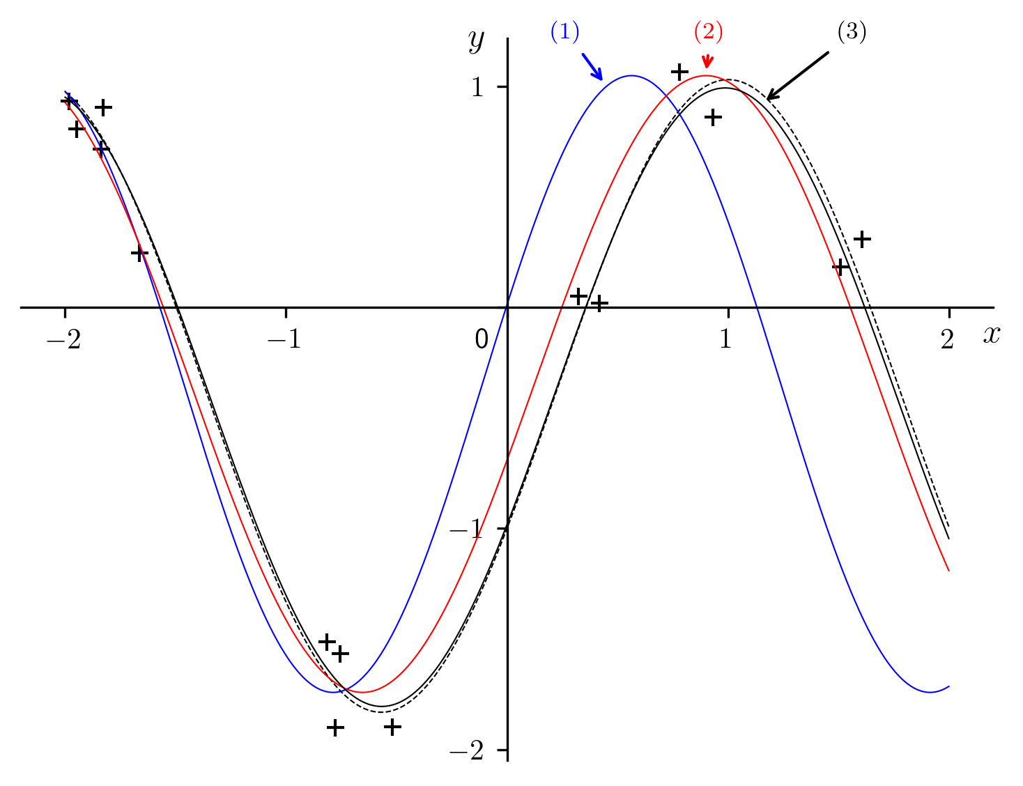
Fig. 14 Regression results for a sample sinusoid.
|
|
|
|
|---|---|---|---|
|
2.32536 | 2.02074 | 2.02074 |
|
-0.345959 | -0.345959 | -0.405617 |
|
1.34913 | 1.35253 | 1.2752 |
|
0.358335 | -0.345283 | -0.577491 |
|
1.39591 | 1.39591 | 1.39987 |
 |
0.25961 | -0.249948 | -0.425231 |
This figure might give the appearance that the prodedure is apparently converging the solid curves with the dotted one with successive approximations. However, attempts to use this approach iteratively would have no effect: repeating the calculations would not modify the final result because it is based on the initial numerical integrations, whose inherent noise will not decrease with further iterations.
Sampling a large number of simulations of different conditions would be
required to form an objective opinion of the properties of this method. We can
refer to Table 12 and Table 13
for a summary of the results for the the optimization of , which
is the essential part of the algorithm. Naturally, the final results are
unchanged from what is shown in Fig. 12 and
Table 13 since  .
.
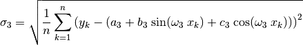
For each simulated value of  , the root mean
square is computed from
, the root mean
square is computed from
(60)
The distribution of  for each fixed value of
is plotted from 10000 simulations, each with a different set of
, since the ordinates are perturbed with a characteristic
root mean square of about the nominal (defined in
Section1). For the plot in figure
for each fixed value of
is plotted from 10000 simulations, each with a different set of
, since the ordinates are perturbed with a characteristic
root mean square of about the nominal (defined in
Section1). For the plot in figure sin-11, the
dispersed ordinates are generated so that the ratio  is always a constant, in this case 0.1. The abscissae, on the other hand, are
generated differently:
is always a constant, in this case 0.1. The abscissae, on the other hand, are
generated differently:
It might seem surprising that the root mean squared error  is
smaller than the initial . The explanation is that the
“optimized” sinusoid will often pass closer to the data points than the “exact”
one, especially with more dispersed points. The differences stem from the
optimization of , which can differ significantly from
, as we saw in Fig. 12 and
Fig. 13. Consequently, for dispersed ordinates, the
error does not increase as significantly as we might have feared in moving away
from uniformly distributed abscissae.
is
smaller than the initial . The explanation is that the
“optimized” sinusoid will often pass closer to the data points than the “exact”
one, especially with more dispersed points. The differences stem from the
optimization of , which can differ significantly from
, as we saw in Fig. 12 and
Fig. 13. Consequently, for dispersed ordinates, the
error does not increase as significantly as we might have feared in moving away
from uniformly distributed abscissae.

Fig. 15 Cumulative distribution functions for the root mean squared error, with uniformly distributed absissae.

Fig. 16 Cumulative distribution functions for the root mean squared error, with non-uniformly distributed absissae.
The biggest difference between the uniform and non-uniform cases is the failure rate of the process. This must be mentioned, since it is the common lot of all methods when the points are irregularly distributed. Inevitably (not frequently, but nevertheless with a non-zero probabililty), we run into data sets in which all the points are tightly clustered. The sinusoid for such data is not defined, and therefore can be neither characterized nor approximated. This can be expressed differently in different portions of the computation, for example through indeterminacy (division by a number too close to zero), non-invertibility of one of the matrices, square root of a negative number, etc.
The calculation of in (52) is where the
majority of failures occur in this method, fortunately quite rarely. For the
hundreds of thousands of simulations performed with uniformly distributed
abscissae, no failure was ever encountered. This is not surprising since the
points could never be clumped in that situation. The case with randomly
selected abscissae, on the other hand, showed a very low failure rate,
dependent on both the dispersion and the quantity of data points under
consideration, as shown in Fig. 17 (which required nearly
five hundred thousand simulations for a coherent view to emerge).

Fig. 17 Failure rates (orders of magnitude).
7. Discussion
Appendix 1: Summary of Sinusoidal Regression Algorithm
Appendix 2: Detailed Procedure for Sinusoidal Regression
Application to the Logistic Distribution (Three Parameters)
Application to the Logistic Distribution (Four Parameters)
Mixed Linear and Sinusoidal Regression
Generalized Sinusoidal Regression
Damped Sinusoidal Regression
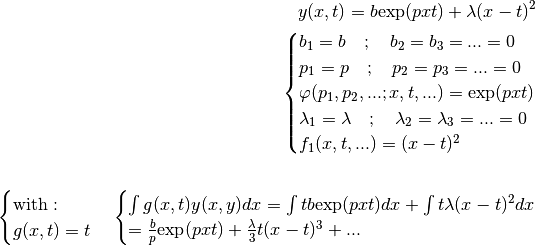
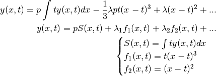
Double Exponential Regression & Double Power Regression
Multivariate Regression
Rather than a single variable, , the objective function depends
on multiple variables,  .
.
Review of the Linear Case
In the simplest case, the function  is linear with respect
to the optimization parameters
is linear with respect
to the optimization parameters
 :
:

The given functions  do not themselves depend on the
optimization parameters.
do not themselves depend on the
optimization parameters.
Given the data points
 [errata-reei-17],
the fitting parameters can be computed using the least-squares method:
[errata-reei-17],
the fitting parameters can be computed using the least-squares method:
With: 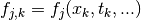
Non-Linear Case
If one or more of the functions depend on the fitting parameter(s), the
corresponding will no longer be linear with respect to the
optimization parameters:

The functions given as  depend on the fitting
parameters
depend on the fitting
parameters  . The complete set of parameters to optimize is
therefore
. The complete set of parameters to optimize is
therefore
 .
The least squares method can not be applied directly in this case. A multitude
of different methods exist, based generally on forming an initial estimate of
the non-linear parameters (), followed by recursive
approximations to progressively optimize the initial guess.
.
The least squares method can not be applied directly in this case. A multitude
of different methods exist, based generally on forming an initial estimate of
the non-linear parameters (), followed by recursive
approximations to progressively optimize the initial guess.
The method studied here follows from a very different principle. We perform
one or more integrations of , for example
 , or
, or  , or
, or
 , or other multiple integrals.
We can can also introduce new functions  , to simplify the
integrals:
, to simplify the
integrals:  , or
, or
 , or
, or
 , or other multiple
integrations.
, or other multiple
integrations.
We can see that the possibilities are endless. It is sometimes possible to form
linear combinations of such equations that cancel out the non linear terms
depending on the parameters .
For Example, consider the following function:
We can see that a linear combination between this equation and the definition
of  can be used to cancel out the term
 :
:
 will be approximated numerically from the data.
This relationship is linear in  . Least squares
regression gives us the desired approximation of
. Least squares
regression gives us the desired approximation of  . This reduces the
equation for to a linear relationship with regards to
and
. This reduces the
equation for to a linear relationship with regards to
and  .
.
Nevertheless, the equations above are not quite correct, as they were
deliberately left incomplete, so as to simplify the following explanation. The
integrals can not be left in their indefinite form, especially when it comes to
numerical integration. It is necessary to define a lower limit if integration.
This requirement does not pose any fundamental difficulty for a function
of one variable. It does, however, become a sensitive problem for
functions of multiple variables. The potential problems
with numerical integration must be examined carefully in the presence of
multiple variables (), even when the integration is only
carried out over one of them.